Clase 4: Deconvolución e Integración con scRNA-seq

Taller de Transcriptómica Espacial

2026-05-20

Resumen: ¿Dónde estamos?

Clases anteriores:

  • Clase 1: Teoría de tecnologías espaciales
  • Clase 2: FASTQs → Space Ranger → Matriz de conteo → QC, clustering, genes espacialmente variables (Seurat + Banksy)
  • Clase 3: Tecnologías espaciales basadas en microscopía (MERFISH)

Hoy:

  • Procesamiento del atlas scRNA-seq (Chromium Flex)
  • Anotación automatizada con Azimuth
  • Deconvolución de Visium HD con spacexr/RCTD
  • Integración con datos Xenium ??

Pregunta central:Clusters espaciales en Visium HD (Banksy) vs ¿qué tipos celulares son?

Necesitamos una referencia anotada.

El diseño experimental del estudio

Del mismo bloque FFPE se generaron secciones seriadas para múltiples plataformas:

Plataforma Resolución Cobertura Pacientes
Visium HD 2–16 µm bins Transcriptoma completo P1, P2, P5 CRC
Chromium Flex Unicelular Transcriptoma completo 5 CRC + 3 NAT
Xenium Subcelular ~500 genes (panel) P1, P2, P4, P5 CRC

Al usar secciones seriadas, los tipos celulares en el scRNA-seq representan fielmente lo que está en el tejido espacial.

Chromium Flex: ¿Qué es?

Diferencias con Chromium 3’/5’:

  • Basado en sondas (como Visium HD), no poly-dT
  • Compatible con FFPE: mismo tejido que el espacial
  • Permite multiplexeo: múltiples muestras en un mismo GEM well
  • Probe barcodes (BC001–BC004) identifican cada muestra

Estructura del multiplexeo:

Pool Muestras
Pool 1 (L1–L4) P2CRC, P4CRC
Pool 2 (L1–L4) P1CRC, P3CRC, P5CRC, P2NAT
Pool 3 (L1–L4) P5NAT, P3NAT

8 muestras × 4 librerías técnicas = 32 combinaciones

Cell Ranger multi demultiplexa por probe barcode, luego aggr combina todo en una sola matriz con sufijos -1 a -32.

Aunque el flex parece más de todas sus tecnologías 💪

Datos descargados de 10x Genomics

Scripts por si es de su interés FlexSingleCell.R ejecutado con slurm script

# Archivos descargados de cf.10xgenomics.com:
# 1. HumanColonCancer_Flex_Multiplex_count_filtered_feature_bc_matrix.tar.gz
# 2. HumanColonCancer_Flex_Multiplex_count_analysis.tar.gz

# Después de descomprimir:
# filtered_feature_bc_matrix/   ← matriz de conteo (MTX)
#   ├── barcodes.tsv.gz          (278,610 barcodes con sufijo -1 a -32)
#   ├── features.tsv.gz
#   └── matrix.mtx.gz
# analysis/
#   └── umap/gene_expression_2_components/projection.csv

¿Por qué MTX y no H5?

Porque lo hice en Ken y requiere hdf5r, que a su vez necesita la librería del sistema HDF5 correctamente configurada. En nuestro cluster, la instalación de HDF5 tenía un path roto. El formato MTX (Matrix Market) se lee con Read10X() sin dependencias adicionales.

Cargando los datos y asignando pacientes

library(Seurat)
library(dplyr)
library(ggplot2)

flex_counts <- Read10X("flex_scrna/filtered_feature_bc_matrix/")
cat("Matrix dim:", dim(flex_counts), "\n")
# 36170 genes × 278610 cells
# El sufijo del barcode (-1 a -32) indica la muestra
# Orden determinado por cellranger aggr
sample_map <- data.frame(
  suffix = 1:32,
  patient = c(
    "P2CRC","P4CRC","P2CRC","P4CRC","P2CRC","P4CRC","P2CRC","P4CRC",
    "P1CRC","P3CRC","P5CRC","P2NAT","P1CRC","P3CRC","P5CRC","P2NAT",
    "P1CRC","P3CRC","P5CRC","P2NAT","P1CRC","P3CRC","P5CRC","P2NAT",
    "P5NAT","P3NAT","P5NAT","P3NAT","P5NAT","P3NAT","P5NAT","P3NAT"),
  tissue = c(
    "CRC","CRC","CRC","CRC","CRC","CRC","CRC","CRC",
    "CRC","CRC","CRC","NAT","CRC","CRC","CRC","NAT",
    "CRC","CRC","CRC","NAT","CRC","CRC","CRC","NAT",
    "NAT","NAT","NAT","NAT","NAT","NAT","NAT","NAT")
)

barcode_suffix <- as.numeric(gsub(".*-(\\d+)$", "\\1", colnames(flex_counts)))
flex <- CreateSeuratObject(counts = flex_counts, project = "ColonCancer_Flex", min.cells = 3)
flex$patient <- sample_map$patient[barcode_suffix]
flex$tissue  <- sample_map$tissue[barcode_suffix]

UMAP de Cell Ranger: ¿Pacientes separados?

Code
# Cell Ranger calcula un UMAP durante el pipeline aggr
umap_cr <- read.csv("flex_scrna/analysis/umap/gene_expression_2_components/projection.csv")
rownames(umap_cr) <- umap_cr$Barcode
umap_cr <- umap_cr[colnames(flex), ]

flex[["umap"]] <- CreateDimReducObject(
  embeddings = as.matrix(umap_cr[, c("UMAP.1", "UMAP.2")]),
  key = "UMAP_", assay = "RNA"
)

DimPlot(flex, group.by = "patient", reduction = "umap", pt.size = 1)

Control de calidad y filtrado

flex[["MT.percent"]] <- PercentageFeatureSet(flex, pattern = "^MT-")

# Umbrales: percentiles 2.5% y 97.5% + MT < 25%
UMI_TH  <- quantile(flex$nCount_RNA,   c(0.025, 0.975))
Gene_TH <- quantile(flex$nFeature_RNA, c(0.025, 0.975))

flex <- subset(flex,
  MT.percent   < 25 &
  nCount_RNA   > UMI_TH[1]  & nCount_RNA   < UMI_TH[2] &
  nFeature_RNA > Gene_TH[1] & nFeature_RNA < Gene_TH[2]
)
cat("Cells after QC:", ncol(flex), "\n")

La estrategia de filtrado es idéntica a la del artículo original: remover el 2.5% extremo en UMIs y genes, más un umbral de 25% para genes mitocondriales.

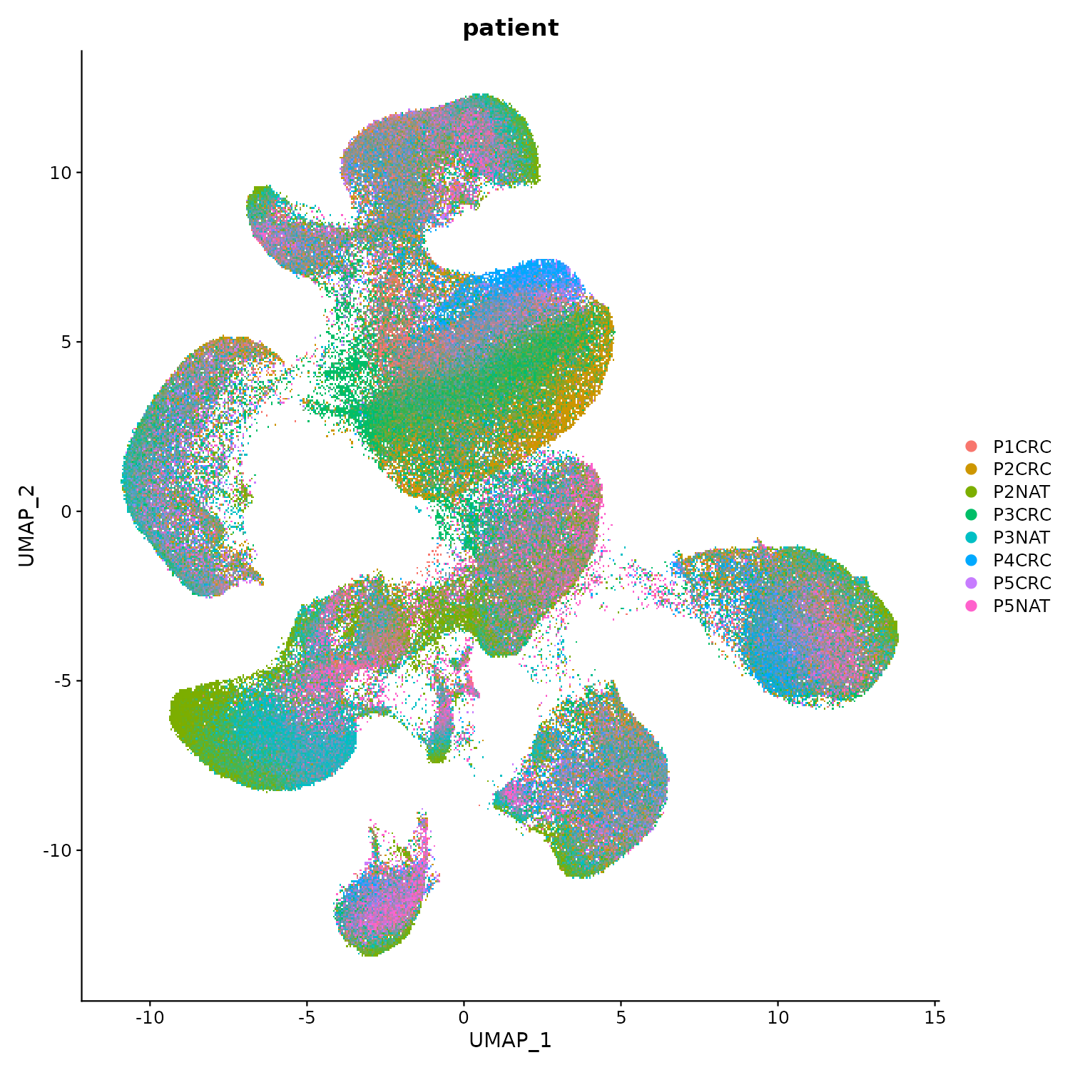
Procesamiento estándar con Seurat

Code
flex <- NormalizeData(flex)
flex <- FindVariableFeatures(flex)
flex <- ScaleData(flex)
flex <- RunPCA(flex)
flex <- FindNeighbors(flex, dims = 1:25)
flex <- FindClusters(flex, resolution = 0.6)
flex <- RunUMAP(flex, dims = 1:25, reduction.name = "umap.seurat")

Clusters de Seurat

Coloreado por paciente

Anotación automatizada con Azimuth

Azimuth es un servicio de anotación automatizada basado en transferencia de etiquetas desde un atlas de referencia pre-anotado.

¿Cómo funciona?

  1. Tu objeto Seurat se envía al servicio en la nube
  2. Se proyecta sobre una referencia (Human Colon)
  3. Regresa con etiquetas de tipo celular + scores de confianza

Niveles de anotación:

  • azimuth_broad → categorías amplias (Immune, Epithelial, Stromal)
  • azimuth_medium → subdivisiones (T cell, B cell, Macrophage)
  • azimuth_fine → tipos específicos (CD8+ TRM, Goblet, CAF)
  • azimuth_label → más detallado
library(AzimuthAPI)

flex <- CloudAzimuth(
  flex,
  assay = "RNA"
)

# Columnas nuevas:
# azimuth_broad
# azimuth_medium
# azimuth_fine
# azimuth_label
# final_level_confidence

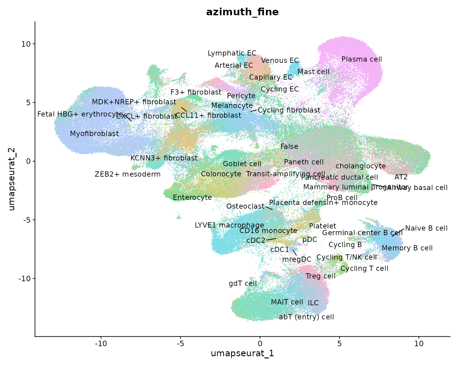
Resultado de Azimuth: anotación fina

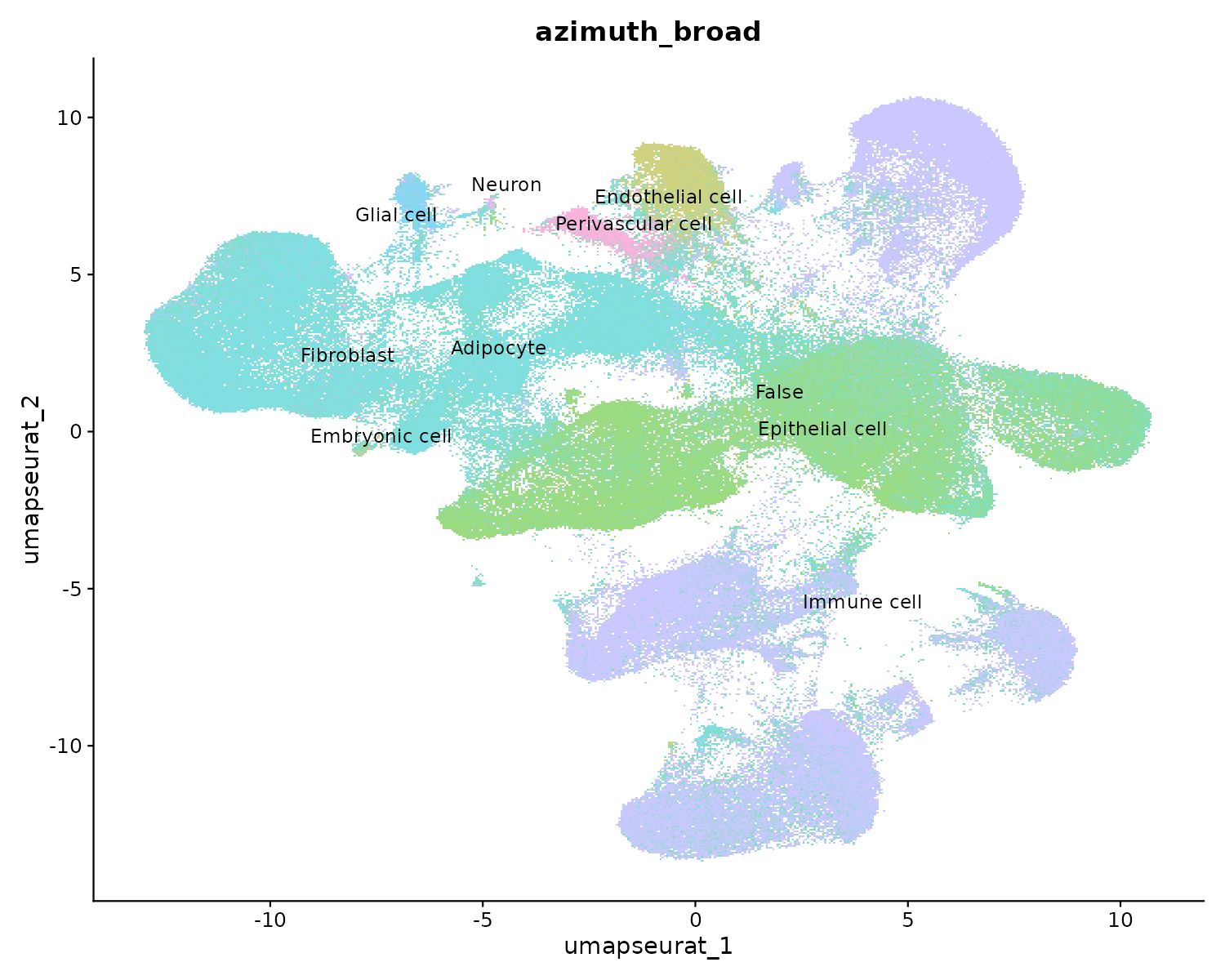
Resultado de Azimuth: anotación amplia

Validación con marcadores canónicos

Code
lineage_markers <- c(
  "EPCAM","KRT8","KRT20","PIGR", "LGR5",          # epitelial
  "CEACAM5","CEACAM6","MUC2",              # tumor / goblet
  "CD3D","CD3E","CD8A","CD4","FOXP3",      # T cells
  "NKG7","GNLY",                           # NK
  "MS4A1","CD79A","JCHAIN","MZB1",         # B / plasma
  "CD68","CD163","CSF1R","LYZ","S100A8",   # mieloides
  "COL1A1","DCN","LUM",                    # fibroblastos
  "PECAM1","VWF","CDH5",                   # endotelial
  "ACTA2","DES","MYH11"                    # músculo liso
)

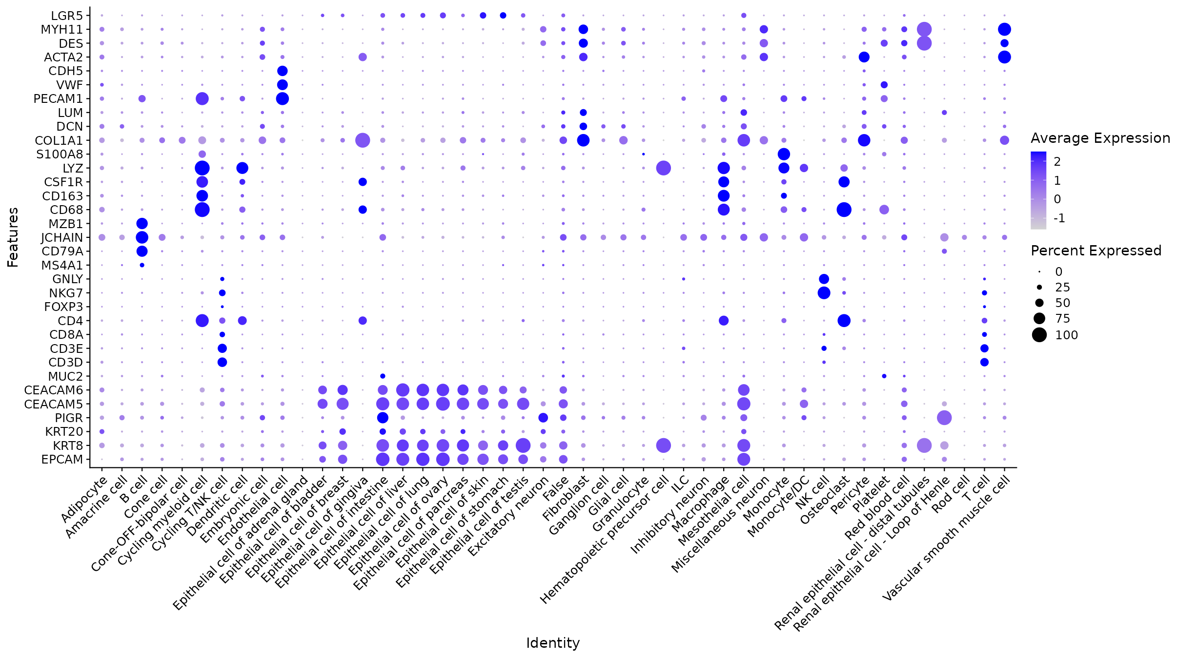
DotPlot: marcadores vs. tipos celulares

FeaturePlot: expresión de marcadores en UMAP

Confianza de la anotación

Score de confianza en UMAP

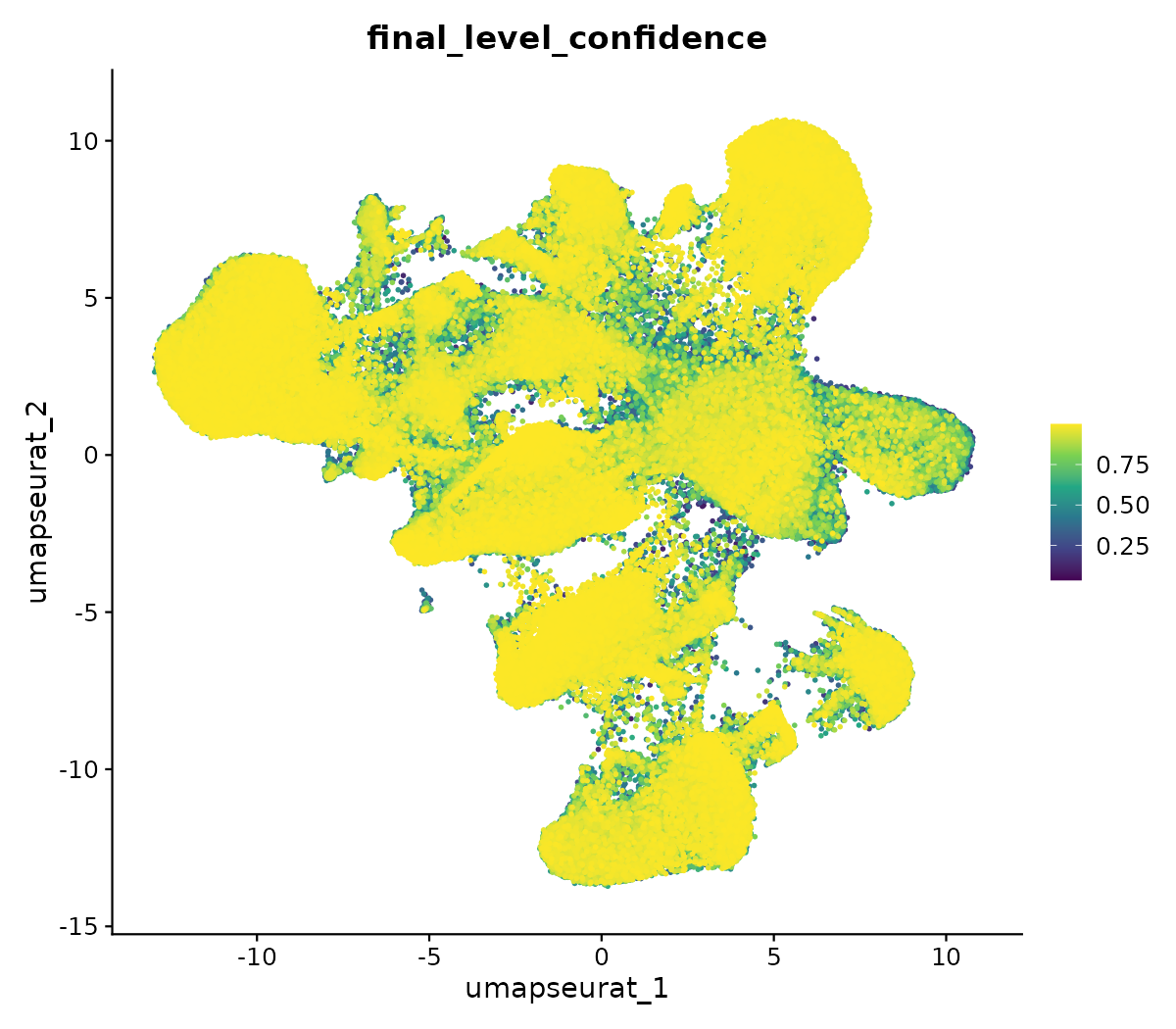
El final_level_confidence indica qué tan segura es la asignación:

  • > 0.8: alta confianza
  • 0.5–0.8: aceptable
  • < 0.5: revisar manualmente

Las células con baja confianza suelen estar en:

  • Transiciones entre tipos
  • Tipos no representados en la referencia
  • Doublets / baja calidad

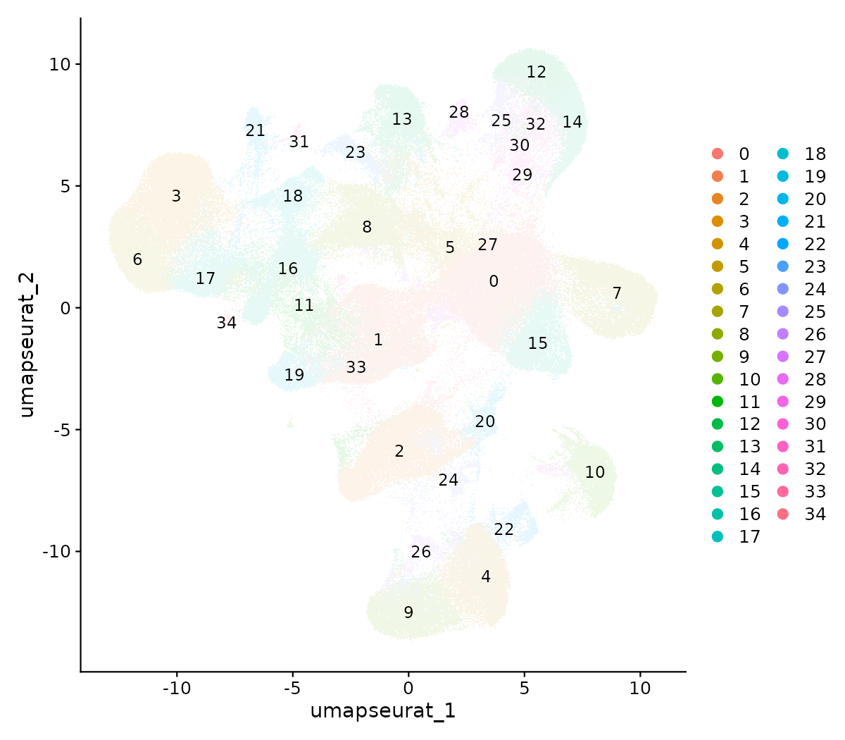
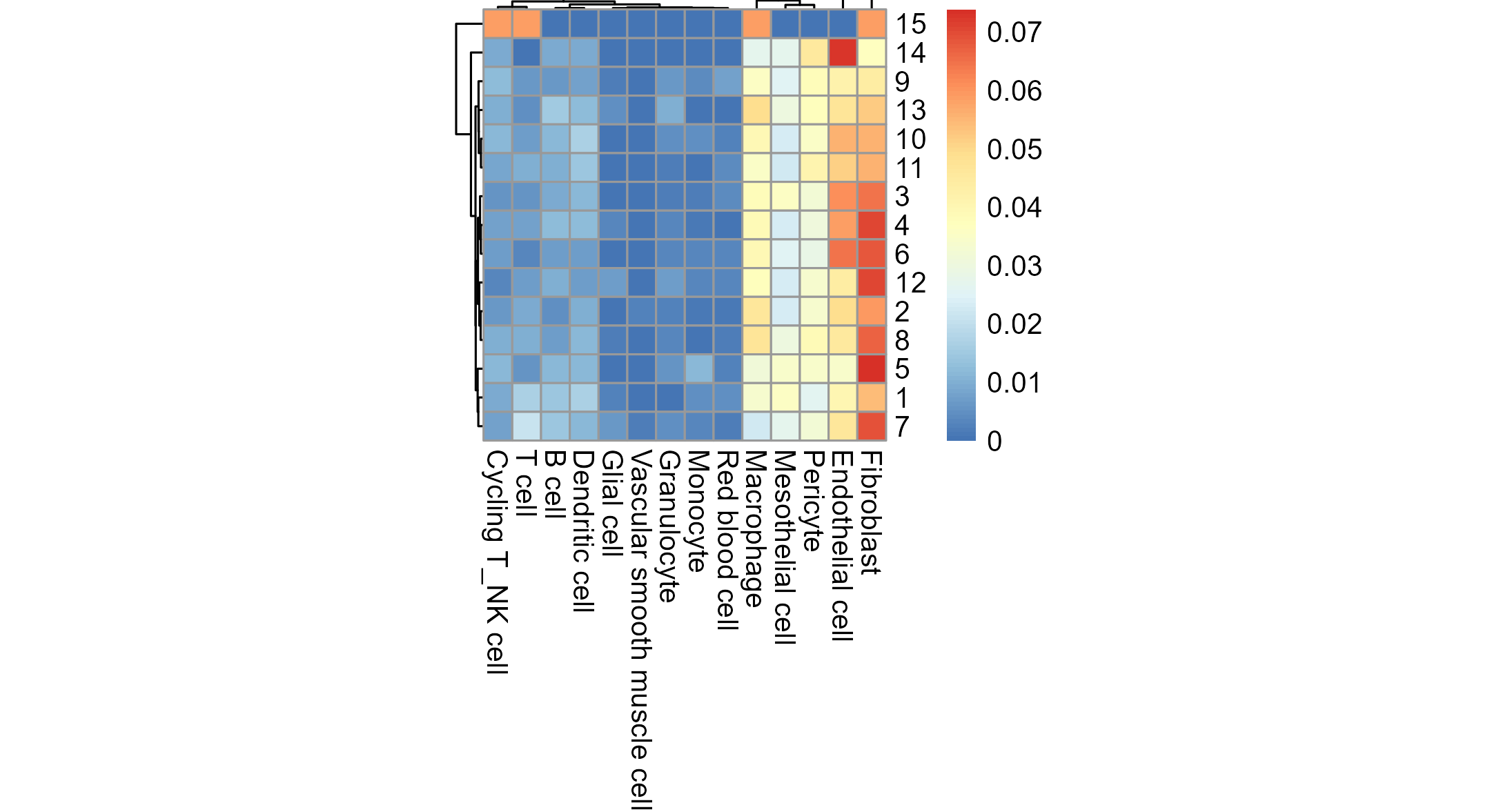
Cluster vs. tipo celular predicho

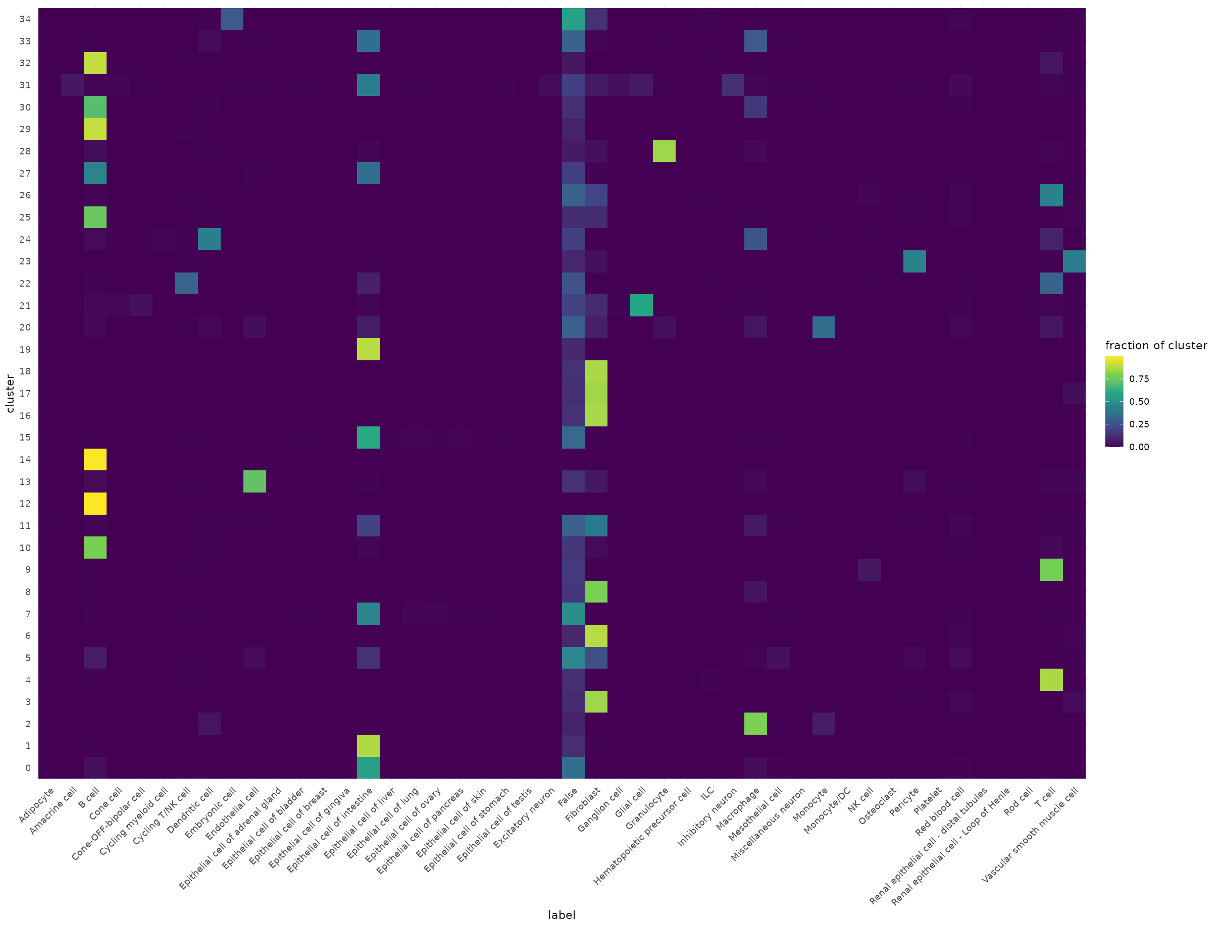
Cada fila es un cluster de Seurat, cada columna un tipo celular predicho por Azimuth. Si un cluster tiene una sola columna dominante, la anotación es consistente.

El objeto anotado: flex_annotated.rds

#saveRDS(flex, "flex_scrna/flex_annotated.rds")

# Para cargarlo en la clase:
flex <- readRDS("flex_scrna/flex_annotated.rds")

# Contiene:
# - Matriz de conteo normalizada (278K → ~250K tras QC)
# - Metadatos: patient, tissue, library
# - Anotaciones: azimuth_broad, azimuth_medium, azimuth_fine, azimuth_label
# - UMAP de Cell Ranger + UMAP de Seurat
# - Clusters de Seurat (resolution 0.6)

Punto de partida

Les entrego flex_annotated.rds con todo lo anterior ya procesado. A partir de aquí, lo usaremos como referencia para deconvolucionar los datos de Visium HD.

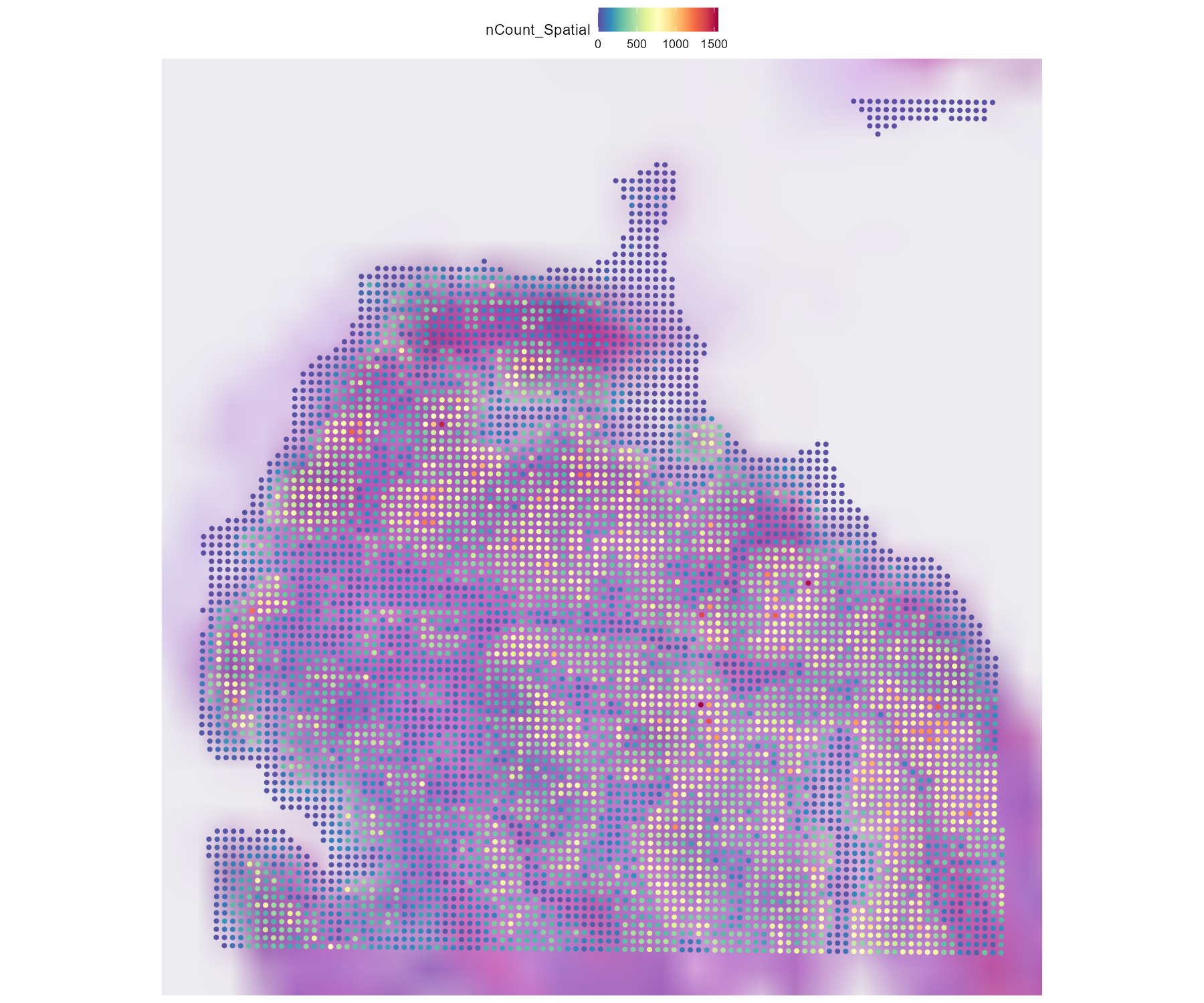
¿Qué es la deconvolución espacial?

Cada bin de Visium HD (8 µm) puede contener 1–2 células. El perfil de expresión del bin es una mezcla de los tipos celulares presentes.

Deconvolución = estimar la composición de tipos celulares por bin, usando el atlas scRNA-seq como referencia.

Herramienta: spacexr / RCTD

  • Robust Cell Type Decomposition
  • Modelo probabilístico que estima proporciones
  • Modo doublet: asume máximo 2 tipos por bin (ideal para 8 µm)

Instalando spacexr con aceleración para Visium HD

El artículo incluye un PR con mejoras de velocidad específicas para datos de alta definición (modo doublet):

  • Paralelización con foreach + doParallel en lugar de makeClusters
  • Vectorización de gather_results (cuello de botella original)
  • Barra de progreso para monitorear el avance
# Instalar desde el PR directamente
pak::pak("dmcable/spacexr#206")

# O desde el fork del autor (Juan Pablo Romero, 10x Genomics)
pak::pak("jpromeror/spacexr@speed_up")

# Dependencias necesarias
install.packages(c("doParallel", "foreach"))

Nota

Esta rama solo acelera el modo doublet. Los modos full y multi no están optimizados todavía. Sinceramente no vi un gran cambio, y en la laptop no corrió por un bug.

Preparando la referencia para RCTD

library(spacexr)

# Cargar el atlas anotado
flex <- readRDS("flex_annotated.rds")

VlnPlot(flex, features = c("CEACAM5", "CEACAM6"), 
        group.by = "azimuth_fine", pt.size = 0) +
  coord_flip()

# Relabel: epithelial cells with high CEACAM5/6 that are patient-specific → Tumor
flex$cell_type_final <- as.character(flex$azimuth_medium)

# Identify which cells express tumor markers
tumor_cells <- colnames(flex)[
  FetchData(flex, "CEACAM5")[,1] > 1 & 
  flex$azimuth_medium %in% c("Epithelial cell of intestine", "Goblet cell")
]
flex$cell_type_final[colnames(flex) %in% tumor_cells] <- "Tumor"

table(flex$cell_type_final) |> sort(decreasing = TRUE)

# Filtrar solo el paciente que corresponde al Visium HD
# (ej. P1CRC si tu Visium HD es P1CRC)
flex_patient <- subset(flex, patient == "P1CRC")

# Remove cells with "False" or NA annotations
valid_cells <- colnames(flex_patient)[
  !is.na(flex_patient$cell_type_final) & 
  flex_patient$cell_type_final != "False"
]
flex_patient <- subset(flex_patient, cells = valid_cells)

# Extraer counts y etiquetas
counts_sc <- GetAssayData(flex_patient, layer = "counts")
cell_types <- flex_patient$cell_type_final

cell_types <- as.factor(gsub("/", "_", flex_patient$cell_type_final))
names(cell_types) <- colnames(flex_patient)
cell_types <- droplevels(cell_types)


ct_counts <- table(cell_types)
keep_types <- names(ct_counts[ct_counts >= 25])
keep_cells <- names(cell_types)[cell_types %in% keep_types]

counts_sc <- counts_sc[, keep_cells]
cell_types <- droplevels(cell_types[keep_cells])

cat("Removed", length(ct_counts) - length(keep_types), "rare cell types\n")
cat("Remaining:", length(keep_types), "cell types,", length(cell_types), "cells\n")


# Crear objeto Reference de spacexr
reference <- Reference(
  counts = counts_sc,
  cell_types = as.factor(cell_types)
)

Cargando y preparando los datos espaciales para RCTD

Code
#En ken, que no tiene hdf5r pero sí RAM
counts <- Read10X(
  "/mnt/data/transcriptomica/jmiranda/sra_visium_hd/P1CRC_GSM8594567_results/outs/binned_outputs/square_016um/filtered_feature_bc_matrix/"
)

visium <- CreateSeuratObject(counts = counts, assay = "Spatial")

library(arrow)
positions <- read_parquet(
  "/mnt/data/transcriptomica/jmiranda/sra_visium_hd/P1CRC_GSM8594567_results/outs/binned_outputs/square_016um/spatial/tissue_positions.parquet"
)

# Match to barcodes in the object
rownames(positions) <- positions$barcode
positions <- positions[colnames(visium), ]

visium$spatial_row <- positions$pxl_row_in_fullres
visium$spatial_col <- positions$pxl_col_in_fullres


coords <- data.frame(
  x = visium$spatial_col,
  y = visium$spatial_row,
  row.names = colnames(visium)
)
Code
# Cargar el objeto Visium HD procesado

visium <- Load10X_Spatial(
  data.dir = "/mnt/data/transcriptomica/jmiranda/sra_visium_hd/P1CRC_GSM8594567_results/outs",
  #En laptop y con HDF5R
  bin.size = 16
)

#Si viene de geo, especificar nombre de archivos
#visium <- Load10X_Spatial(data.dir = "P1CRC_GSM8594567_results/outs/binned_outputs/square_016um", filename = "filtered_feature_bc_matrix.h5", image.name = "tissue_lowres_image.png")

# Extraer counts y coordenadas
coords <- GetTissueCoordinates(visium)

Subsetting opcional para que no tarde tanto

(De la clase 2)

Code
count.plot <- SpatialFeaturePlot(object, features = "nCount_Spatial") +
  theme(legend.position = "right")
# Extract everything we need
plot_data <- ggplot_build(count.plot)$data[[1]]

x_cuts <- seq(min(plot_data$x), max(plot_data$x), length.out = 9)
y_cuts <- seq(min(plot_data$y), max(plot_data$y), length.out = 9)

ggplot(plot_data, aes(x = x, y = y, color = fill)) +
  geom_point(size = 0.1, shape = 15) +
  scale_color_identity() +
  # Grid
  annotate("segment",
    x = x_cuts, xend = x_cuts,
    y = min(plot_data$y), yend = max(plot_data$y),
    color = "white", linewidth = 0.3, linetype = "dashed") +
  annotate("segment",
    x = min(plot_data$x), xend = max(plot_data$x),
    y = y_cuts, yend = y_cuts,
    color = "white", linewidth = 0.3, linetype = "dashed") +
  # Column labels
  annotate("text",
    x = head(x_cuts, -1) + diff(x_cuts) / 2,
    y = rep(max(plot_data$y) + 5, 8),
    label = 1:8, color = "yellow", size = 3, fontface = "bold") +
  # Row labels
  annotate("text",
    x = rep(min(plot_data$x) - 5, 8),
    y = head(y_cuts, -1) + diff(y_cuts) / 2,
    label = LETTERS[1:8], color = "yellow", size = 3, fontface = "bold") +
  coord_fixed(clip = "off") +
  theme_void() +
  theme(legend.position = "none",
        plot.background = element_rect(fill = "black", color = NA))

Elijan un bloque (o no, pero tardará más)

plot_data$cell <- colnames(object)

# Function to pick a block
pick_block <- function(row_letter, col_number, plot_data, x_cuts, y_cuts) {
  r <- match(toupper(row_letter), LETTERS)
  c <- col_number
  cells <- plot_data$cell[
    plot_data$x >= x_cuts[c] & plot_data$x < x_cuts[c + 1] &
    plot_data$y >= y_cuts[r] & plot_data$y < y_cuts[r + 1]
  ]
  return(cells)
}

# 
cells_block <- pick_block("C", 1, plot_data, x_cuts, y_cuts)
object <- subset(object, cells = cells_block)
#cat("Bins in block D3:", ncol(object_block), "\n")

SpatialFeaturePlot(object, features = "nCount_Spatial", pt.size.factor = 20)

Corriendo deconvolucion

# Crear objeto SpatialRNA de spacexr
counts_spatial <- GetAssayData(visium, layer = "counts")
spatial_rna <- SpatialRNA(
  coords = coords,
  counts = counts_spatial
)

# Crear y ejecutar RCTD

rctd <- create.RCTD(spatial_rna, reference, max_cores = 30)
rctd <- run.RCTD(rctd, doublet_mode = "doublet")
# doublet_mode: máximo 2 tipos por bin (apropiado para 8 µm)

saveRDS(rctd, "resultsRCTD_P1CRC.rds")

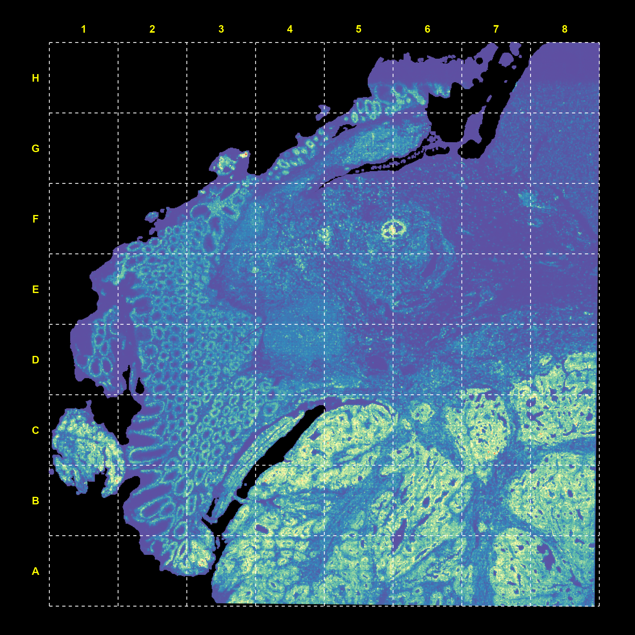
Visualizando la deconvolución

Code
# Extraer los resultados
rctd <- readRDS("resultsRCTD_P1CRC.rds")
results <- rctd@results

# Para modo doublet: tipo celular 1 y 2 por bin + proporciones
cell_type_1 <- results$results_df$first_type
#weirdly stored as scond_type (sic)
cell_type_2 <- results$results_df$scond_type

visium$rctd_class <- results$results_df$spot_class
visium$rctd_weight1 <- results$weights_doublet[, "first_type"]

# Agregar al objeto Seurat
visium$rctd_type1 <- cell_type_1
visium$rctd_type2 <- cell_type_2

# Visualizar el tipo celular dominante
coords <- data.frame(
  x = visium$spatial_col,
  y = visium$spatial_row,
  type = visium$rctd_type1,
  class = visium$rctd_class
)


coords_good <- coords[coords$class != "reject", ]

p <- ggplot(coords_good, aes(x = x, y = -y, color = type)) +
  geom_point(size = 0.1, shape = 15) +
  coord_fixed() +
  theme_minimal() +
  theme(axis.title = element_blank(), axis.text = element_blank()) +
  guides(color = guide_legend(override.aes = list(size = 3))) +
  labs(title = "RCTD deconvolution — dominant cell type")

ggsave("rctd_spatial_celltypes.png", p, width = 12, height = 10, dpi = 150)
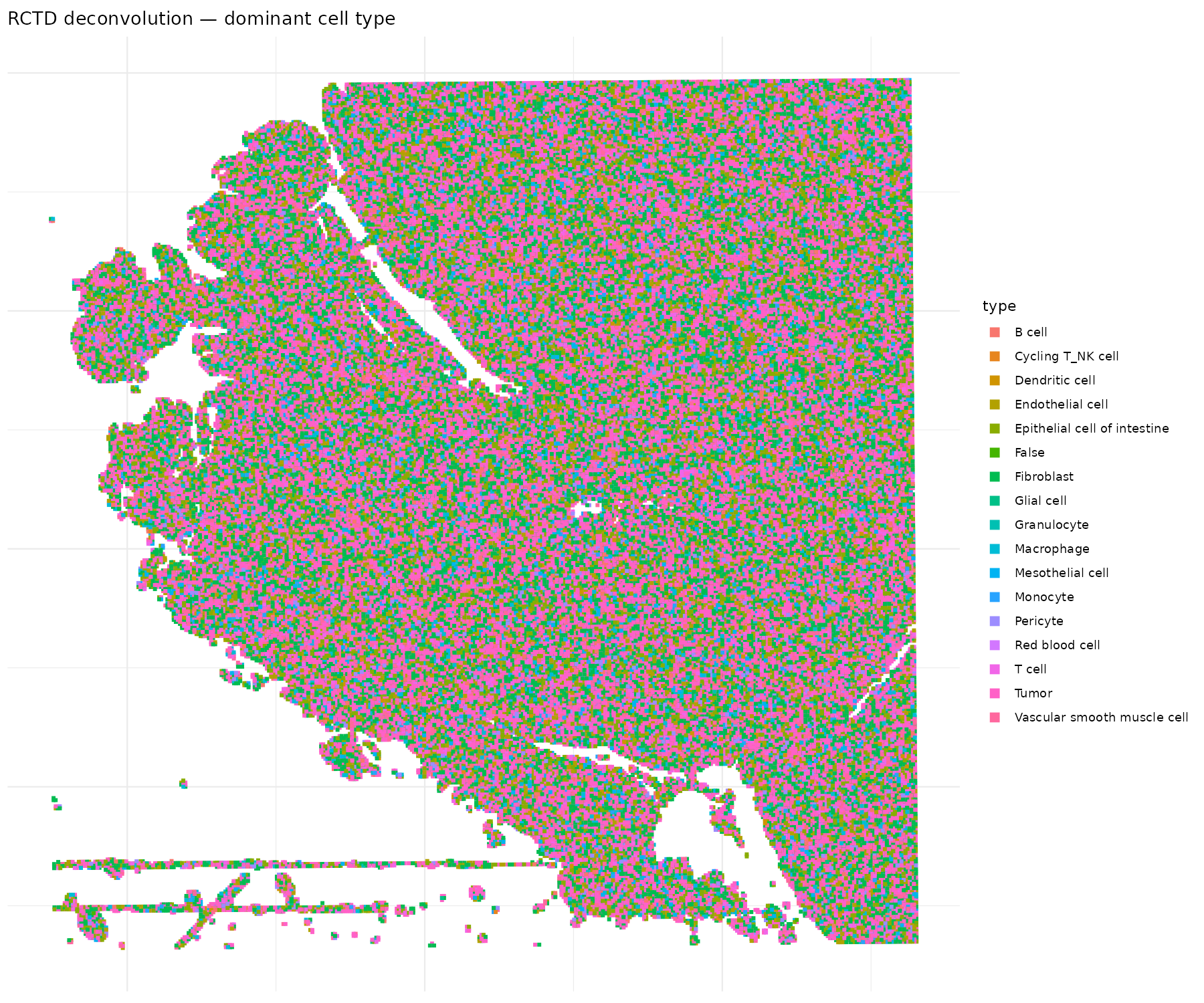
O por paneles

Code
library(patchwork)
weights <- as.data.frame(results$weights)
colnames(weights) <- gsub(" ", "_", colnames(weights))  # spaces break metadata
for (ct in colnames(weights)) {
  visium[[ct]] <- weights[[ct]]
}

# Plot helper using your spatial coords
plot_weight <- function(obj, feature) {
  df <- data.frame(
    x = obj$spatial_col,
    y = obj$spatial_row,
    val = obj[[feature, drop = TRUE]]
  )
  ggplot(df, aes(x = x, y = -y, color = val)) +
    geom_point(size = 0.3, shape = 15) +
    coord_fixed() +
    labs(title = feature, color = NULL) +
    theme_void() +
    theme(plot.title = element_text(size = 9, hjust = 0.5))
}

ct_names <- colnames(weights)

p <- lapply(ct_names, \(ct) plot_weight(visium, ct)) |>
  wrap_plots(nrow = 2, guides = "collect") &
  scale_color_gradientn(colors = rev(hcl.colors(9, "Rocket"))) &
  theme(
    legend.key.width = unit(0.5, "lines"),
    legend.key.height = unit(1, "lines")
  )

ggsave("rctd_all_weights_panels.png", p, width = 20, height = 10, dpi = 150)
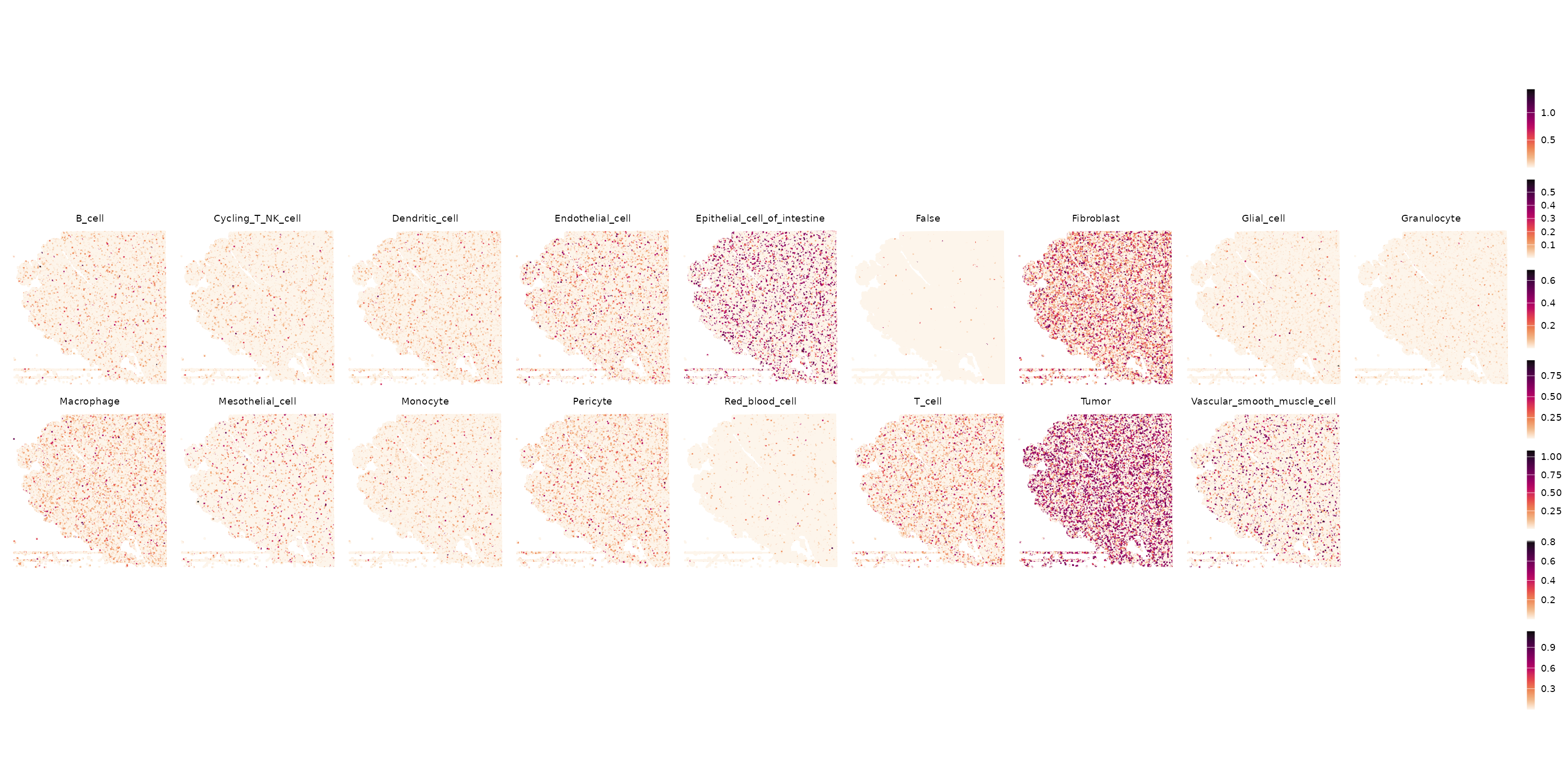
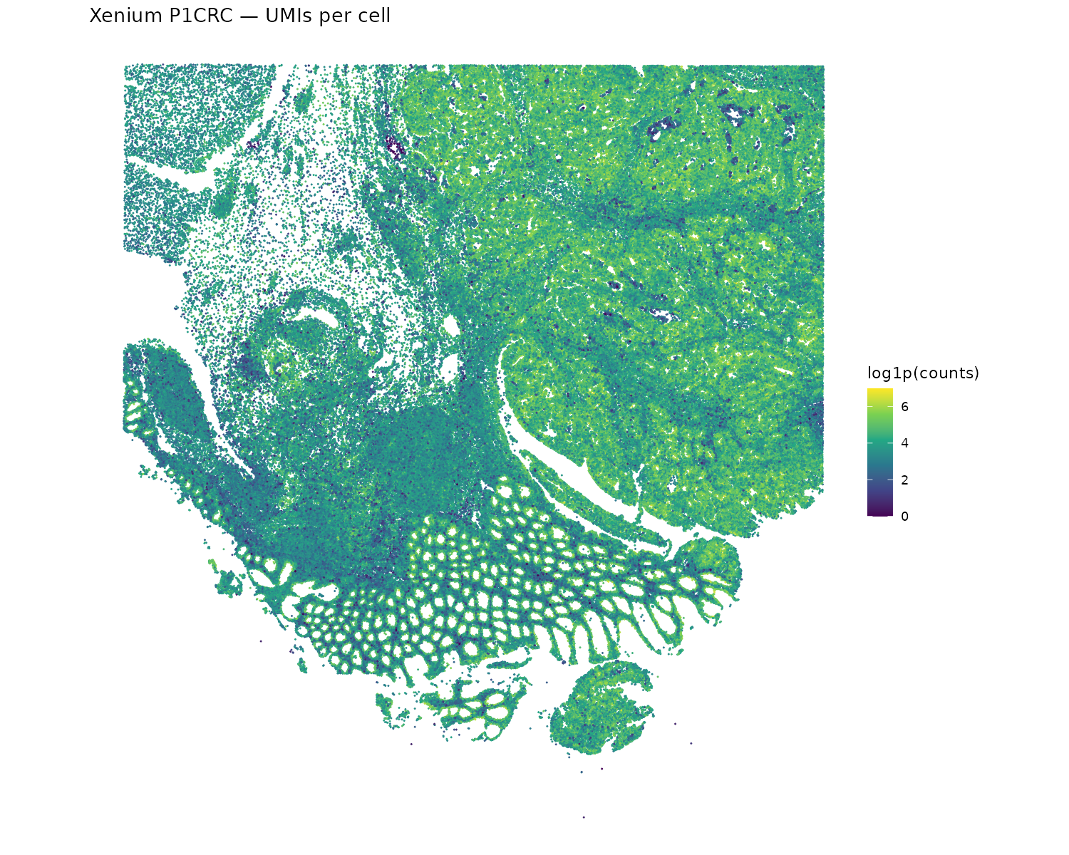
Igual que hace dos clases usamos Banksy (clustering spatial aware)

Transformar seurat a spatial exp

Code
library(SpatialExperiment)
coords <- GetTissueCoordinates(visium)
object_export <- visium

sce <- as.SingleCellExperiment(object_export)
spe <- SpatialExperiment(
  assays = assays(sce),
  colData = colData(sce),
  spatialCoords = as.matrix(coords[colnames(sce), 1:2])
)
#Quitar los ceros
spe <- spe[, colSums(counts(spe)) > 0]
Code
library(Banksy)
library(scuttle)
library(scran)
spe <- logNormCounts(spe)
dec <- modelGeneVar(spe)
hvg <- getTopHVGs(dec, n=3e3)
# set seed for random number generation
# in order to make results reproducible
set.seed(112358)
# 'Banksy' parameter settings
k <- 8   # consider first order neighbors
l <- 0.2 # use little spatial information
a <- "logcounts"
xy <- c("array_row", "array_col")
# restrict to selected features
tmp <- spe[hvg, ]

# compute spatially aware 'Banksy' PCs
tmp <- computeBanksy(tmp, assay_name=a, coord_names=xy, k_geom=k)
tmp <- runBanksyPCA(tmp, lambda=l, npcs=20)
reducedDim(spe, "PCA") <- reducedDim(tmp)
## run UMAP (for visualization purposes only)
# .vhd16 <- runUMAP(.vhd16, dimred="PCA")
# build cellular shared nearest-neighbor (SNN) graph
g <- buildSNNGraph(spe, use.dimred="PCA", type="jaccard", k=20)
# cluster using Leiden community detection algorithm
k <- cluster_leiden(g, objective_function="modularity", resolution=2.5)
table(spe$Banksy <- factor(k$membership))
spe$in_tissue <- TRUE

plotCoords(spe, annotate = "Banksy", point_size = 2, point_shape = 15)

Comparar deconvolución con Banksy

Code
# Get common barcodes (strip -1 suffix if needed)
barcodes_spe <- colnames(spe)
barcodes_seurat <- colnames(visium)

common <- intersect(barcodes_spe, barcodes_seurat)
cat("Common barcodes:", length(common), "\n")

# If 0, check if one has -1 suffix and the other doesn't
# head(barcodes_spe); head(barcodes_seurat)

# Build the cross-table
banksy <- spe$Banksy[match(common, colnames(spe))]
decon <- visium$rctd_type1[match(common, colnames(visium))]

fq <- prop.table(table(banksy, decon), 1)
pheatmap(fq[,-c(5)], cellwidth = 10, cellheight = 10, 
         treeheight_row = 5, treeheight_col = 5)

Xenium: validación ortogonal

¿Por qué Xenium?

  • Resolución subcelular real (no bins)
  • Detección in situ de transcritos individuales
  • Panel de ~500 genes seleccionados

Complementa a Visium HD:

  • Visium HD: transcriptoma completo, resolución bin
  • Xenium: panel limitado, resolución subcelular

Los autores encontraron genes como SELENOP y JCHAIN que no estaban en el panel Xenium original, pero fueron identificados como relevantes gracias a Visium HD → los añadieron como panel Add-on.

# Los datos Xenium se descargaron
# de GEO (GSE280314)
# Contienen:
# - transcripts.csv.gz
# - cells.csv.gz
# - cell_feature_matrix/
# - cell_boundaries/

# Cargar en Seurat:
library(arrow)

# Load transcript-level data
tx <- read_parquet("xenium_data/P1CRC_xenium/transcripts.parquet")
head(tx)
# Should have: x_location, y_location, feature_name, cell_id, etc.

# Load the cell feature matrix (already extracted)
counts <- Read10X("xenium_data/P1CRC_xenium/cell_feature_matrix/")

# If it's a list (multiple feature types), grab the gene expression one
if (is.list(counts)) {
  names(counts)
  counts <- counts[["Gene Expression"]]
}

# Build a basic Seurat object
xenium <- CreateSeuratObject(counts = counts, assay = "Xenium")

# Get per-cell coordinates from transcripts
# (average x,y of all transcripts assigned to each cell)
cell_coords <- tx |>
  dplyr::filter(cell_id != "UNASSIGNED") |>
  dplyr::group_by(cell_id) |>
  dplyr::summarise(x = median(x_location), y = median(y_location), .groups = "drop") |>
  as.data.frame()
rownames(cell_coords) <- cell_coords$cell_id

# Match to barcodes in the object
common <- intersect(colnames(xenium), cell_coords$cell_id)
xenium <- subset(xenium, cells = common)
cell_coords <- cell_coords[colnames(xenium), ]

xenium$x_centroid <- cell_coords$x
xenium$y_centroid <- cell_coords$y

cat("Xenium cells:", ncol(xenium), "\n")
cat("Genes in panel:", nrow(xenium), "\n")

Xenium

Code
df <- data.frame(
  x = xenium$x_centroid,
  y = xenium$y_centroid,
  counts = xenium$nCount_Xenium
)

p <- ggplot(df, aes(x = x, y = -y, color = log1p(counts))) +
  geom_point(size = 0.05) +
  scale_color_viridis_c() +
  coord_fixed() +
  theme_void() +
  labs(title = "Xenium P1CRC — UMIs per cell")

ggsave("xenium_P1CRC_counts.png", width = 10, height = 8, dpi = 150)

Hallazgos principales del estudio

Subpoblaciones de macrófagos:

  1. Pro-tumorales — dos subpoblaciones con perfiles distintos, localizadas en regiones tumorales específicas
  2. Anti-tumorales (SELENOP⁺ C1QC⁺) — colocalizados con células T clonalmente expandidas

Expansión clonal de T cells:

  • Identificaron clonotipos expandidos de CD8⁺ T cells
  • Estos T cells se localizan cerca de macrófagos anti-tumorales y células CEACAM5⁺ tumorales

Sólo posible con datos espaciales:

  • scRNA-seq identifica los tipos celulares
  • Visium HD revela dónde están y con quién interactúan
  • Xenium valida a resolución subcelular

Lección metodológica:

Ninguna plataforma sola responde todas las preguntas. La integración de múltiples modalidades (Visium HD + Flex + Xenium) da el panorama completo.

Actividad práctica

Si quieren aquí o con mejor conexión. En laptop o en clústers (ken o fenix)

  1. Cargar flex_annotated.rds como referencia
    1. Pero sin tumor (Ver diapo: Preparando la referencia para RCTD)
  2. Cargar su objeto Visium HD procesado (de la clase 3, o pueden encontrarlos en mi carpeta de Ken)
  3. Ejecutar RCTD para deconvolucionar su paciente (con 16mum y 30 cores tarda alrededor de 2 horas, try as slurm job).
  4. Visualizar el mapa de tipos celulares en el espacio
  5. Comparar con los clusters de Banksy

Recursos computacionales

RCTD en modo doublet sobre ~500K bins puede tardar >60 minutos y requiere ~16 GB de RAM (el pull request de spacexr no parece haber ayudado). Si su laptop no lo soporta, usen los bins de 16 µm o la subregión (block) que seleccionaron en la clase anterior.

Referencias

¡Gracias! La última clase es de ustedes