Clase 11 - 09 abril 2025

Author

Jero

Cargando librerias

Cargamos varias librerias del tidyverse para hacernos más facil la vida con los dataframes. Cargamos Seurat para hacer la manipulacion de los datos de scRNA-seq.

suppressPackageStartupMessages(library(Seurat))
library(tidyr)
library(readr)
suppressPackageStartupMessages(library(dplyr))
suppressPackageStartupMessages(library(magrittr))
library(stringr)
library(stats)
library("RColorBrewer")
library(ggplot2)
library(ggfortify)

Recuerden que si hace falta una librería, se puede instalar con el comando install.packages(““) y hay que poner el nombre de la librería entre comillas:

install.packages("ggfortify")

Warning: Paket 'ggfortify' wird gerade benutzt und deshab nicht installiert

Cargando archivos

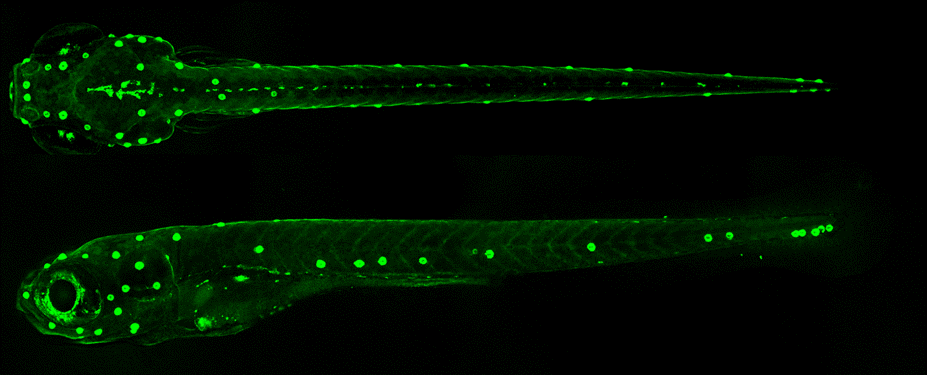
Los datos vienen del artículo (Kozak et al. 2020) donde se secuenciaron los transcriptomás de células del neuromasto de pez cebra por dos técnicas diferentes, concentrándonos en un tipo celular específico, las hair cells. Los archivos son open source y se pueden encontrar en SCRB y 10X Chromium.¹

Localización de los neuromastos en el pez cebra

Hair cells

Acá quizás tengan que cambiar el path si los archivos no están dentro de una carpeta llamada “data”.

hc10x <- LoadSeuratRds("data/haircells10X_clase9.RDS")

Support cells

sc10x <- LoadSeuratRds("data/supportcells10X_clase9.RDS")

Hair cells con una tecnica de single cell alternativa

hcSCRB <- LoadSeuratRds("data/haircells1SCRB_clase9.RDS")

Exploración

Los archivos ya fueron filtrados. En hc10x@metadata hay features extra para cada célula, por ejemplo, el número de transcritos expresados, el número de moléculas de RNA detectadas, y qué porcentaje de éstos pertenecen a transcritos mitocondriales, ribosomales, de hemoglobina o EGFP.

VlnPlot(hc10x, features = c("nFeature_RNA", "nCount_RNA", "percent.mt", "percent.ribo", "percent.hemo", "EGFP"), ncol = 3)

Algunas de las distribuciones están truncadas porque filtramos los valores extremos de acuerdo a valores de MADS, una especie de desviación estandard basada en la media, como se sugiere en https://www.sc-best-practices.org/preprocessing_visualization/quality_control.html#filtering-low-quality-cells

Adicionalmente, se corrigió el “background” de la sopa de RNA usando la libreria SoupX y se clasificaron algunas células como dobletes basado en el algoritmo de la librería scDblFinder. Para más info, ver la referencia anterior.

El score de dobletes correlaciona con la cantidad de RNA detectado y el número de genes.

#FeatureScatter(hc10x, feature1 = "log1p_nCount", feature2 = "log1p_nGenes")
hc10x@meta.data %>% ggplot(aes(log1p_nCount, log1p_nGenes, col = scDblFinder_score)) + geom_point() + theme_bw()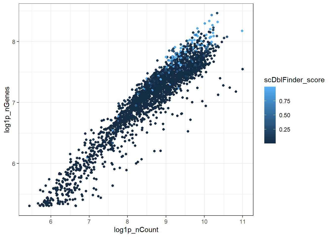

La correción de SoupX sólo tiene sentido con técnicas basadas en microfluidos como 10X Chromium. La tecnica SCRB no involucra una “sopa”, la librería de cDNA se hace para cada célula individual y no hay ninguna célula en este dataset con un número suficientemente bajo de lecturas para calcular la sopa.

El cálculo de dobletes tiene más sentido porque las células del neuromasto son difíciles de disociar completamente. El porcentaje de dobletes correlaciona con el número de células porque es una función de la velocidad a la que pasan las células en la corriente de microfluidos, ya sea en el aparato de 10X o en el FACS (SCRB).

Porcentaje de dobletes en SCRB:

#Hair cells SCRB
(tab <- (hcSCRB@meta.data$scDblFinder_class %>% table))

.
singlet doublet 
    178       6

#Porcentaje
purrr::reduce(rev(tab), `/`) * 100

[1] 3.370787

#Hair cells 10X
(tab <- (hc10x@meta.data$scDblFinder_class %>% table))

.
singlet doublet 
   2679     140

#Porcentaje
purrr::reduce(rev(tab), `/`) * 100

[1] 5.225831

#Support cells
(tab <- sc10x@meta.data$scDblFinder_class %>% table)

.
singlet doublet 
   7899     836

purrr::reduce(rev(tab), `/`) * 100

[1] 10.58362

	Singles	Dobletes	Porcentaje
Hair cells SCRB	178	6	3.37
Hair cells 10X	2679	140	5.22
Support cells 10X	7899	836	10.5

Normalización y pipeline standard con Seurat

hc10x <- NormalizeData(hc10x)

Normalizing layer: counts

hc10x <- FindVariableFeatures(hc10x)

Finding variable features for layer counts

hc10x <- ScaleData(hc10x)

Centering and scaling data matrix

hc10x <- RunPCA(hc10x)

PC_ 1 
Positive:  ttc36, bhmt, pah, pcbd1, LOC100537277, hpdb, si:dkey-12l12.1-1, slc16a10, c1qtnf5, ecrg4a 
       ucp1, LOC100535731, tspan18b, fah, qdpra, notum1b, mxra8b, plpp3, and2, serpine2 
       prrx1a, twist1a, tmem176, gstz1, kazald3, mxra8a, timp2a-1, twist3, col1a1a, ptx3a 
Negative:  zgc:111983, icn2, si:ch211-207n23.2, cldne, lye, mid1ip1a, si:ch211-95j8.2, si:ch211-195b11.3, krt17, dhrs13a.2 
       si:dkey-247k7.2, anxa1b, LOC100535170, si:ch211-117m20.5, si:ch211-157c3.4, anxa1c, elovl7b, si:ch73-204p21.2, si:dkey-87o1.2, hrc 
       zgc:163030, si:ch73-52f15.5, agr1, zgc:193505, soul2, cd9b, si:dkey-222n6.2, plekhf1, LOC101882496, tmem176l.4 
PC_ 2 
Positive:  aldob, sepp1a-1, zgc:85975, cd63, sepp1a, pah, mgst1.2, ttc36, si:dkey-12l12.1-1, f3b 
       ecrg4a, and2, LOC100537277, slc16a10, sept9a, c1qtnf5, fah, msx2b, LOC100535731, bambia 
       tspan18b, pcbd1, zgc:111983, hpdb, lye, msx1b, notum1b, si:ch211-95j8.2, icn2, cldne 
Negative:  s100t, anxa5a, zgc:109934, zgc:173594, s100s, transEGFP, wu:fj16a03, zgc:171713, tuba1a, si:dkey-222f2.1 
       zgc:173593, LOC100006428, tuba1c, zgc:101772, LOC558816, rasd1, barhl1a, mt2, pcp4b, adcyap1b 
       zgc:195356, zgc:55461, nkx3.2, meig1-1, zgc:198419, zgc:55461-1, gstp1, atp1a1b, LOC101884954-1, barhl1a-2 
PC_ 3 
Positive:  fcer1gl, zgc:64051, LOC100151049, si:ch211-102c2.4, ncf1, LOC100537803, zgc:153073, si:dkey-27i16.2, ccr9a, samsn1a 
       il1b, spi1b, arpc1b, si:dkey-262k9.4, srgn-1, wasb, cmklr1, ctss2.1, lcp1, LOC100536989 
       spi1a, grap2b, ptpn6, ppp1r18, LOC100536213-1, LOC108180725, si:dkey-53k12.2, cd83, si:dkey-5n18.1, plek 
Negative:  krt5, wu:fb18f06, s100t, zgc:109934, anxa5a, zgc:173594, s100s, zgc:171713, wu:fj16a03, transEGFP 
       si:dkey-222f2.1, tuba1a, zgc:173593, LOC100006428, zgc:101772, tuba1c, LOC558816, cyt1, zgc:92242, barhl1a 
       rasd1, zgc:153665, abcb5, cyt1l, pcp4b, si:ch211-105c13.3, krtt1c19e, zgc:195356, krt4-1, zgc:153911 
PC_ 4 
Positive:  cldn1, col17a1a, si:ch1073-406l10.2, cxl34b.11, epgn, zgc:136930, col1a2, mmp30, rbp4, col1a1b 
       si:dkey-183i3.5, zgc:86896, krt91, pfn1, col11a1a, crp4, ptgdsb.1, krtt1c19e, spaca4l, tmsb1 
       postnb, cfd-2, itgb4, sparc, LOC100331704, tmsb4x, lgals1l1, si:dkey-102c8.3, LOC100538177, si:dkey-33c14.3 
Negative:  gstp1, s100t, anxa5a, zgc:109934, mdh1aa, zgc:171713, zgc:173594, s100s, si:dkey-222f2.1, txn 
       transEGFP, tuba1a, zgc:173593, wu:fj16a03, tuba1c, LOC100006428, zgc:101772, rasd1, abcb5, LOC558816 
       zgc:153665, mt2, barhl1a, zgc:153911, cd82a, si:ch211-98n17.5-1, si:dkeyp-110c7.4, rtn4b, nkx3.2, hmgn2 
PC_ 5 
Positive:  tnnc2, ckma, ckmb, aldoab, atp2a1, acta1b, tpma, tnnt3b, myl1, actn3a 
       tnni2a.4, mylz3, smyd1a, mybphb, myoz1b, actc1b, mylpfb, nme2b.2, pvalb2, tmod4 
       tmem38a, atp2a1l, LOC100007086-1, slc25a4-1, LOC100537702, ldb3b, mylpfa-2, ampd1, pvalb1, ckmt2b 
Negative:  zgc:171713, s100t, si:dkey-222f2.1, gstp1, zgc:109934, anxa5a, si:dkeyp-110c7.4, tuba1a, zgc:173594, transEGFP 
       zgc:173593, s100s, si:dkey-205h13.2, cbln18, si:dkey-4p15.5, cbln20, LOC100536887, wu:fj16a03, LOC100147871, txn 
       zgc:101772, tuba1c, LOC100006428, LOC100329486, si:dkey-33m11.8, negaly6, si:ch73-199e17.1, LOC558816, krt1-c5, nkx3.2

hc10x <- FindNeighbors(hc10x, dims = 1:30)

Computing nearest neighbor graph

Computing SNN

hc10x <- FindClusters(hc10x)

Modularity Optimizer version 1.3.0 by Ludo Waltman and Nees Jan van Eck

Number of nodes: 2819
Number of edges: 103587

Running Louvain algorithm...
Maximum modularity in 10 random starts: 0.8682
Number of communities: 19
Elapsed time: 0 seconds

“Inspired by these earlier applications, we define a new similarity between two data points based on the ranking of their shared neighborhood” (Xu and Su 2015).

hc10x <- RunUMAP(hc10x, dims = 1:30)

Warning: The default method for RunUMAP has changed from calling Python UMAP via reticulate to the R-native UWOT using the cosine metric
To use Python UMAP via reticulate, set umap.method to 'umap-learn' and metric to 'correlation'
This message will be shown once per session

10:48:52 UMAP embedding parameters a = 0.9922 b = 1.112

10:48:52 Read 2819 rows and found 30 numeric columns

10:48:52 Using Annoy for neighbor search, n_neighbors = 30

10:48:52 Building Annoy index with metric = cosine, n_trees = 50

0%   10   20   30   40   50   60   70   80   90   100%

[----|----|----|----|----|----|----|----|----|----|

**************************************************|
10:48:53 Writing NN index file to temp file C:\Users\mwaso\AppData\Local\Temp\RtmpmiAn33\file7a8c31a93132
10:48:53 Searching Annoy index using 1 thread, search_k = 3000
10:48:54 Annoy recall = 100%
10:48:54 Commencing smooth kNN distance calibration using 1 thread with target n_neighbors = 30
10:48:55 Initializing from normalized Laplacian + noise (using RSpectra)
10:48:55 Commencing optimization for 500 epochs, with 114940 positive edges
10:49:07 Optimization finished

DimPlot(hc10x, group.by = c("seurat_clusters"), reduction = "umap")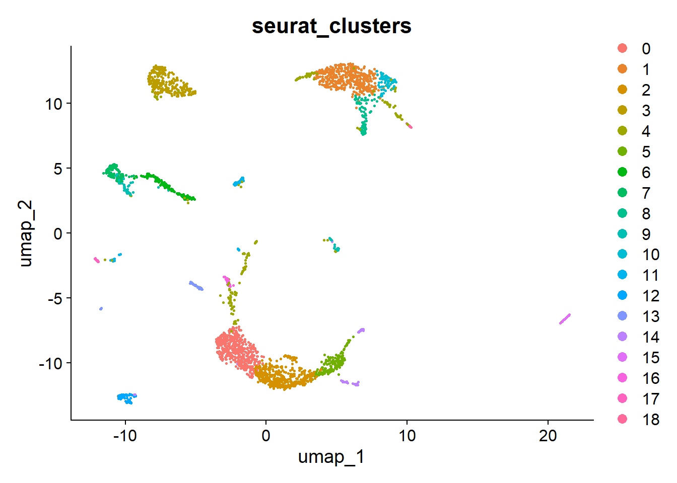

Integración para anotación

Por suerte, para el pez cebra ya existe una referencia de datos de single cell en diferentes etapas del desarrollo: Zebrafish atlas. Los datasets originales se distribuyen en el formato AnnData que usa el ecosistema de scanpy, pero es posible convertirlos a Seurat con:

(No correr este codigo)

library(zellconverter)
sce <- zellconverter::readH5AD("zf_atlas_5dpf_v4_release.h5ad")
as.Seurat(sce, counts = "counts", data = "X")

zf_atlas5dpf <- LoadSeuratRds("data/zf_atlas_5dpf_v4_release.RDS")
plot <- DimPlot(zf_atlas5dpf, reduction = "X_umap", group.by = "zebrafish_anatomy_ontology_class") + NoLegend()
LabelClusters(plot = plot, id = "zebrafish_anatomy_ontology_class")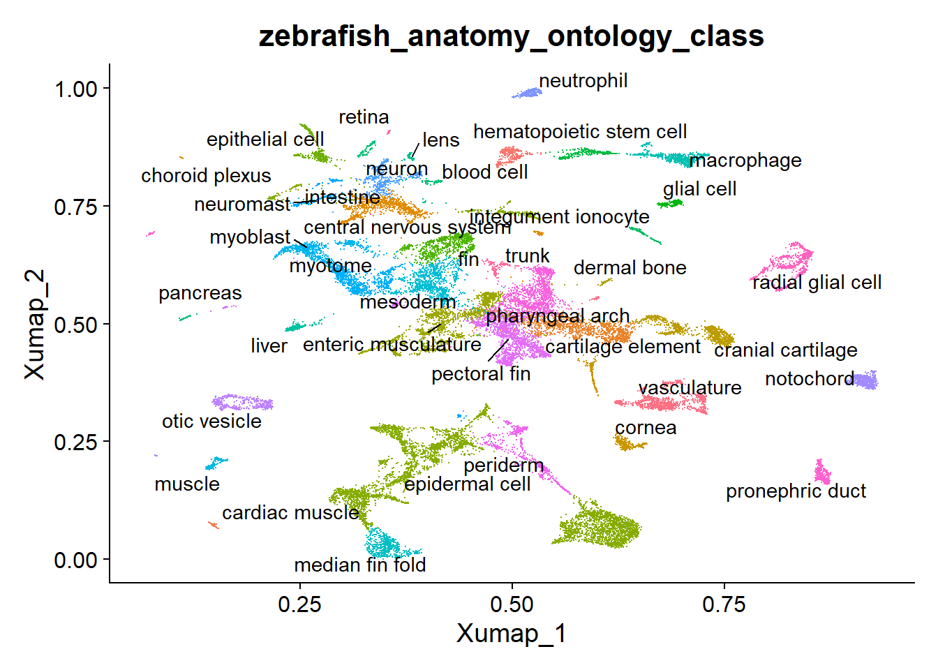

La referencia del atlas ya viene con umap, clusters y normalización calculada. Sin embargo, para este pipeline, necesitamos calcular los componentes principales para integrar con nuestros datos, también hay que re-calcular el UMAP porque usaremos el modelo resultante posteriormente.

#Los datos en data ya estan normalizados
#zf_atlas5dpf <- NormalizeData(zf_atlas5dpf)
zf_atlas5dpf <- FindVariableFeatures(zf_atlas5dpf)
zf_atlas5dpf <- ScaleData(zf_atlas5dpf)

Centering and scaling data matrix

zf_atlas5dpf <- RunPCA(zf_atlas5dpf)

PC_ 1 
Positive:  si:dkey-194e6.1, pdzk1ip1, BX530068.1, cx32.3, cdh17, pdzk1, si:ch211-139a5.9, g6pca.2, epdl2, slc2a11l 
       acy3.2, fbp1b, cubn, eps8l3a, dpys, slc22a6l, hoga1, ezra, slc23a1, eps8l3b 
       slc22a7b.1, slc26a1, cox6a2, grhprb, cdaa, slc2a11a, ggt1b, npr1b, pnp6, slc2a2 
Negative:  krt4, cyt1, icn2, anxa1b, dhrs13a.2, ppl, evpla, si:ch211-125o16.4, cyt1l, abcb5 
       si:ch211-195b11.3, cldne, mid1ip1a, si:dkey-222n6.2, scel, zgc:193505, si:dkey-247k7.2, agr1, zgc:111983, si:dkeyp-51b9.3 
       si:ch211-157c3.4, znf185, si:ch211-207n23.2, si:cabz01007794.1, stard14, abca12, icn, si:dkey-202l22.6, krt17, s100w 
PC_ 2 
Positive:  sparc, tmsb4x, col1a2, rbp4, col1a1a, dcn, col1a1b, actc1b, fmoda, rgs5a 
       ptgdsb.1, hpdb, soul5, zgc:153704, si:ch211-156j16.1, cnmd, glula, eno1a, pvalb2, col9a2 
       col2a1a, tgfbi, vim, ttn.2, CR318588.4, rbp5, apoa2, cxcl12a, col9a3, ecrg4a 
Negative:  dhrs13a.2, evpla, anxa1b, icn2, si:ch211-125o16.4, abcb5, cldne, ppl, stard14, si:ch211-195b11.3 
       si:dkey-247k7.2, agr1, si:ch211-207n23.2, scel, znf185, zgc:193505, zgc:111983, si:dkey-222n6.2, si:ch211-157c3.4, mid1ip1a 
       si:dkeyp-51b9.3, si:cabz01007794.1, krt4, cyt1l, abca12, zgc:100868, si:dkey-202l22.6, cyt1, soul2, krt17 
PC_ 3 
Positive:  apoa1b, abcb11b, apoa2, zgc:112265, cfhl4, fgb, fga, c3a.1, si:ch211-212c13.8, CR626907.1 
       cfb, apoba, si:dkey-105h12.2, vtnb, fgg, c3a.2, serpinc1, itih2, cp, c3b.2 
       si:ch1073-464p5.5, ambp, a2ml, gc, serpinf2a, apom, c9, ces2a, si:ch211-288g17.4, serpina1 
Negative:  fcer1gl, spi1b, si:dkey-5n18.1, mpeg1.1, laptm5, plxnc1, ptprc, coro1a, wasb, lcp1 
       itgae.1, ctss2.2, ctss2.1, MFAP4-3, havcr1, slc22a21, si:ch211-147m6.1, il1b, grna, cmklr1 
       fcer1g, si:ch211-194m7.3, ccr9a, ccl34b.1, marco, ctsl.1, si:ch211-194m7.4, rgs13, c1qb, ptpn6 
PC_ 4 
Positive:  abcb11b, zgc:171534, cfb, apoa2, apoa1b, cfhl4, fgb, CR626907.1, cfh, si:dkey-105h12.2 
       serpinf2a, zgc:112265, fga, apoba, itih2, si:ch211-212c13.8, a2ml, c3a.1, fgg, si:ch211-288g17.4 
       shbg, serpinc1, cp, vtnb, c3b.2, c3a.2, zgc:172051, ambp, si:ch73-281k2.5, apom 
Negative:  srl, desma, tmem38a, cav3, ldb3b, acta1a, casq2, atp2a1, txlnba, si:ch211-266g18.10 
       obscnb, SRL, actn3b, cavin4a, klhl31, ckmb, ryr1a, neb, trdn, myom1a 
       txlnbb, prx, aldoab, pvalb4, obsl1b, CABZ01072309.2, tnnt3a, ldb3a, CABZ01078594.1, tpm2 
PC_ 5 
Positive:  srl, desma, tmem38a, casq2, ldb3b, txlnba, si:ch211-266g18.10, actn3b, SRL, cavin4a 
       acta1a, atp2a1, cav3, obscnb, aldoab, klhl31, ryr1a, ckmb, trdn, myom1a 
       txlnbb, neb, zgc:171534, nme2b.2, pvalb4, arpp21, cfh, obsl1b, abcb11b, cfb 
Negative:  sparc, col11a1a, ptgdsb.1, si:dkey-194e6.1, col9a2, cnmd, col1a1a, col9a3, si:ch211-139a5.9, lrp2a 
       col1a2, pdzk1ip1, col2a1a, slc2a11l, cdh17, cubn, pdzk1, slc20a1a, slc22a6l, col11a2 
       zgc:175280, col1a1b, acy3.2, epyc, slc22a7b.1, slc2a11a, ucmab, slc26a1, slc23a1, pnp6

#zf_atlas5dpf <- FindNeighbors(zf_atlas5dpf)
#zf_atlas5dpf <- FindClusters(zf_atlas5dpf)
zf_atlas5dpf <- RunUMAP(zf_atlas5dpf, dims = 1:30, reduction = "pca", return.model = T)

UMAP will return its model

10:49:55 UMAP embedding parameters a = 0.9922 b = 1.112

10:49:55 Read 24987 rows and found 30 numeric columns

10:49:55 Using Annoy for neighbor search, n_neighbors = 30

10:49:55 Building Annoy index with metric = cosine, n_trees = 50

0%   10   20   30   40   50   60   70   80   90   100%

[----|----|----|----|----|----|----|----|----|----|

**************************************************|
10:50:01 Writing NN index file to temp file C:\Users\mwaso\AppData\Local\Temp\RtmpmiAn33\file7a8c1c9969dd
10:50:01 Searching Annoy index using 1 thread, search_k = 3000
10:50:17 Annoy recall = 100%
10:50:17 Commencing smooth kNN distance calibration using 1 thread with target n_neighbors = 30
10:50:19 Initializing from normalized Laplacian + noise (using RSpectra)
10:50:22 Commencing optimization for 200 epochs, with 1120824 positive edges
10:51:03 Optimization finished

Podemos usar esto como un filtro de cuales células son del tejido de interés y cuales no. En este caso, podemos ver que hay un sobrelape entre las células que expresan el transgénico y las células del neuromasto.

#Creamos un objeto con las células ancla, pares de células en comun entre ambos datasets
hc_anchors <- FindTransferAnchors(reference = zf_atlas5dpf, query = hc10x, dims = 1:30, reference.reduction = "pca")

Projecting cell embeddings

Finding neighborhoods

Finding anchors

    Found 2297 anchors

predictions <- TransferData(anchorset = hc_anchors, refdata = zf_atlas5dpf$zebrafish_anatomy_ontology_class, dims = 1:30)

Finding integration vectors

Finding integration vector weights

Predicting cell labels

hc10x <- AddMetaData(hc10x, metadata = predictions)
plot2 <- FeaturePlot(hc10x, reduction =  "umap", features = c("transEGFP") )
plot <- DimPlot(hc10x, reduction = "umap", group.by = "predicted.id") + NoLegend()
LabelClusters(plot = plot, id = "predicted.id") + plot2

Esta es otra manera de visualizar lo anterior, en este caso, proyectamos las células experimentales sobre las coordenadas de UMAP del atlas orginal.

hc10x <- MapQuery(anchorset = hc_anchors, reference = zf_atlas5dpf, query = hc10x, refdata = zf_atlas5dpf$zebrafish_anatomy_ontology_class, reference.reduction = "pca", reduction.model = "umap")

Finding integration vectors

Finding integration vector weights

Predicting cell labels

Warning: Layer counts isn't present in the assay object; returning NULL
Warning: Layer counts isn't present in the assay object; returning NULL
Warning: Layer counts isn't present in the assay object; returning NULL


Integrating dataset 2 with reference dataset

Finding integration vectors

Integrating data

Computing nearest neighbors

Running UMAP projection

10:51:50 Read 2819 rows

10:51:50 Processing block 1 of 1

10:51:50 Commencing smooth kNN distance calibration using 1 thread with target n_neighbors = 30
10:51:50 Initializing by weighted average of neighbor coordinates using 1 thread
10:51:50 Commencing optimization for 67 epochs, with 84570 positive edges
10:51:52 Finished

p1 <- DimPlot(zf_atlas5dpf, reduction = "umap", group.by = "zebrafish_anatomy_ontology_class", label = T, repel = T) + NoLegend()
p2 <- DimPlot(hc10x, reduction = "ref.umap", group.by = "predicted.id", label = T, repel = T) + NoLegend()

p1 + p2

Warning: ggrepel: 1 unlabeled data points (too many overlaps). Consider
increasing max.overlaps

Warning: ggrepel: 1 unlabeled data points (too many overlaps). Consider
increasing max.overlaps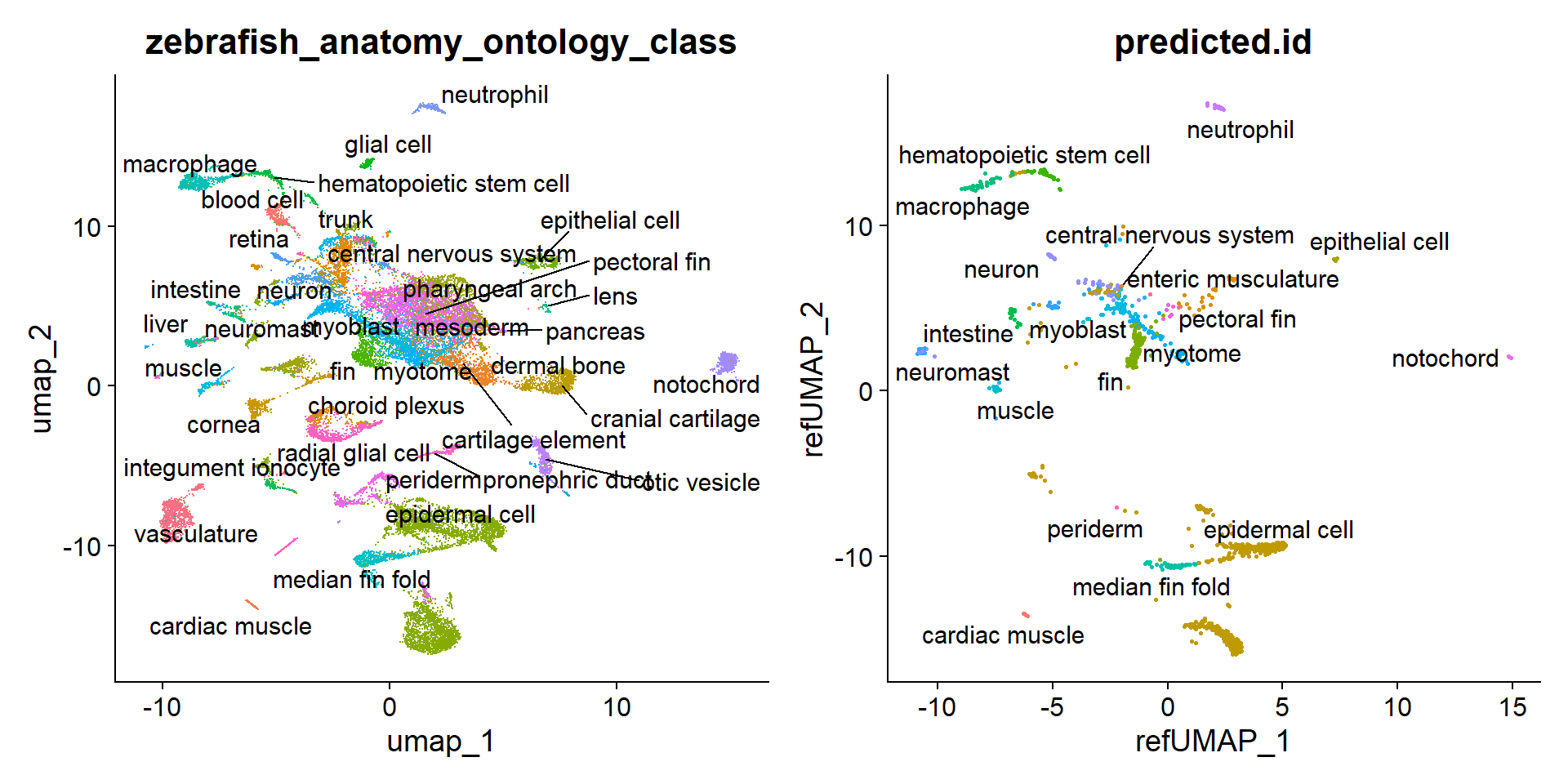

Es un poco engañoso, el tamaño de los clústers representados en el UMAP no necesariamente representa el número de células de cada uno. De hecho, las células del neuromasto representan el grupo mayoritario con 1123 de 2819 células.

hc10x[["predicted.id"]] %>% table

predicted.id
         cardiac muscle  central nervous system     enteric musculature 
                      7                       1                      27 
         epidermal cell         epithelial cell                     fin 
                   1008                       4                     261 
hematopoietic stem cell               intestine              macrophage 
                     30                      26                      37 
        median fin fold                  muscle                myoblast 
                     46                      41                      55 
                myotome               neuromast                  neuron 
                     52                    1123                      66 
             neutrophil               notochord            pectoral fin 
                     23                       3                       6 
               periderm         pharyngeal arch 
                      1                       2

La correlacion entre las probabilidad de ser neuromasto y la expresion del trangénico es alta. El clúster de 0 expresion de transEGFP pero alta probabilidad de neuromasto, ilustra una de las limitantes de scRNA-seq: no todos los genes expresados se detectan en el 100% de las células.

FeatureScatter(hc10x, "transEGFP", "prediction.score.neuromast", smooth = T, group.by = "predicted.id", slot = "data")

Warning: The `<scale>` argument of `guides()` cannot be `FALSE`. Use "none" instead as
of ggplot2 3.3.4.
ℹ The deprecated feature was likely used in the Seurat package.
  Please report the issue at <https://github.com/satijalab/seurat/issues>.

Warning: The dot-dot notation (`..density..`) was deprecated in ggplot2 3.4.0.
ℹ Please use `after_stat(density)` instead.
ℹ The deprecated feature was likely used in the Seurat package.
  Please report the issue at <https://github.com/satijalab/seurat/issues>.

Anotando las SCRB hair cells

Tambien vamos a anotar las hair cells de la tecnica de pozos, una variante de SCRB optimizada y open source (Bagnoli et al. 2018).

hcSCRB <- NormalizeData(hcSCRB)

Normalizing layer: counts

hcSCRB <- FindVariableFeatures(hcSCRB)

Finding variable features for layer counts

hcSCRB <- ScaleData(hcSCRB)

Centering and scaling data matrix

hcSCRB <- RunPCA(hcSCRB)

PC_ 1 
Positive:  zgc:193811, si:dkey-250d21.1, pcp4b, seh1l, alg11, mapre2, emx2, osbpl5, phf20b, b9d2 
       mcu, mgst3a, cirbpb, fam49bb, pfn2l, zgc:101569, cbln20, dedd1, sptssa, bloc1s2 
       tmem18, gmfb, stx5al, eif4a1a, blcap, pcgf1, cyb5d1, tmed2, tomm22, apbb3 
Negative:  vipb, egr4, hpcal4, phox2bb, LOC110438943-1, atp1b3a, hand2, nalcn, si:ch73-71c20.5, zgc:158463 
       kif1ab, arrdc2, si:dkeyp-115e12.6-1, gap43, LOC100005446, rpl17, lin37, LOC795227, arid6, kif26aa 
       ap4m1, spout1, zgc:55461, nf2a, LOC110439214, coa7, star, si:dkey-6n6.2, LOC108191643, krt91 
PC_ 2 
Positive:  vipb, hand2, LOC110439214, wu:fj16a03, si:dkey-6n6.2, star, atp1b3a, spout1, adcyap1b, hpcal4 
       phox2bb, akap17a, kif26aa, ap4m1, si:ch73-1a9.3, coa7, stx12, plxna4, LOC795227, arid6 
       zmp:0000001301, fam206a, rnf150a, spg21, nup107, arrdc2, pdcd5, snrpd2, zgc:136930, skida1 
Negative:  slc1a3a, si:dkey-205h13.2, LOC100147871, si:dkey-4p15.5, cbln18, foxq1a, phlda2, LOC100536887, si:dkeyp-110c7.4, si:dkey-33m11.8 
       cbln20, zgc:77517, add3a, LOC101886389, zgc:171713, zgc:77517-1, LOC100329486, mbnl2, si:ch73-347e22.8, lfng 
       junba, igfbp1a, fndc7a, si:ch211-195b11.3, abca12, LOC563933, cldnb, chrna7, aqp3a, sdc2 
PC_ 3 
Positive:  LOC100005446, hpcal4, tsr3, ap4m1, nalcn, atp1b3a, kif26aa, skida1, pgm1, LOC795227 
       hand2, spout1, grnb, si:dkeyp-68b7.7, dlc1, star, arrdc2, nf2a, bhmt, atp13a1 
       supt6h, ywhag2-1, aim1b, si:dkey-6n6.2, gap43, znf408, eif2b1, ak4, zc4h2, LOC101882691 
Negative:  zgc:152830, zbed4, dpm3, mrc1a, acin1b, kitlga, mbnl2, abca12, csrnp1b, hif1al 
       ccng2, ehbp1, rad50, snapin, copg2, rabif, lcor, gid8a, si:ch211-253h3.1, dhrs4 
       fam110b, ccdc127b, si:dkey-34l15.1-1, itgb4, ddx39b, zgc:158463, adkb, gale, wu:fc21g02, LOC110439372 
PC_ 4 
Positive:  LOC108190653, nalcn, itgb4, gap43, ap4m1, hpcal4, grb10a, si:ch73-71c20.5, spout1, LOC795227 
       kif26aa, hand2, atp1b3a, gng12a, smurf1, LOC100005446, trmt13, si:dkeyp-115e12.6-1, star, LOC101887000 
       coa7, gpr78b, aim1b, LOC100329486, stox2b, lcor, dlc1, nf2a, mgst2, skida1 
Negative:  zgc:55461, mrps11, si:ch211-148l7.4, rplp2l, rtca, rassf2a, dynlt3, ptmab, gstp1, rps20 
       si:ch211-236g6.1, LOC110440166, ccdc135, tcea2, LOC101885587, zgc:66433, dlx4b, ubiad1, shisa2a, dnase1l4.1 
       pigs, tmem30ab, sap30bp, pwwp2b, si:ch73-52e5.1, transEGFP, rpl27, zgc:110046, rps9, lmo7b 
PC_ 5 
Positive:  dhtkd1, inpp4aa, clstn1, dnase1l1, tdrd3, spg11, clrn2, prrc2c, si:zfos-1011f11.1, cadm4 
       si:ch73-347e22.8, mrpl13, soul2, zfyve9a, laptm4a, nup93, sdc2, ube3c, pak2a, zcchc9 
       actl6a, si:dkey-286j15.1-1, ago2, chrna7, eif3ja, hs6st2, wu:fi15d04, ppp6r3, cldnb, kmt2e 
Negative:  LOC108190653, gsnb, gale, grb10a, tbc1d17, ppp5c, arl13b, lcor, crebrf, zgc:162344 
       rpap3, arhgap32a, dfna5b, mgst2, si:ch211-39i22.1, zbed4, timm23a, si:ch73-111k22.3, si:dkey-46g23.1, rbm28 
       itgb4, tprb, dapk3, dhrs4, phb, abhd15a, uqcc2, copb2, urm1, lmo7b

hcSCRB <- FindNeighbors(hcSCRB)

Computing nearest neighbor graph

Computing SNN

hcSCRB <- FindClusters(hcSCRB)

Modularity Optimizer version 1.3.0 by Ludo Waltman and Nees Jan van Eck

Number of nodes: 184
Number of edges: 6821

Running Louvain algorithm...
Maximum modularity in 10 random starts: 0.5791
Number of communities: 2
Elapsed time: 0 seconds

hcSCRB <- RunUMAP(hcSCRB, dims = 1:30, reduction = "pca", return.model = T)

UMAP will return its model

10:52:06 UMAP embedding parameters a = 0.9922 b = 1.112

10:52:06 Read 184 rows and found 30 numeric columns

10:52:06 Using Annoy for neighbor search, n_neighbors = 30

10:52:06 Building Annoy index with metric = cosine, n_trees = 50

0%   10   20   30   40   50   60   70   80   90   100%

[----|----|----|----|----|----|----|----|----|----|

**************************************************|
10:52:06 Writing NN index file to temp file C:\Users\mwaso\AppData\Local\Temp\RtmpmiAn33\file7a8c36e81516
10:52:06 Searching Annoy index using 1 thread, search_k = 3000
10:52:06 Annoy recall = 100%
10:52:06 Commencing smooth kNN distance calibration using 1 thread with target n_neighbors = 30
10:52:07 Initializing from normalized Laplacian + noise (using RSpectra)
10:52:07 Commencing optimization for 500 epochs, with 6864 positive edges
10:52:08 Optimization finished

La técnica de pozos gana en términos de especificidad. El 100% de las células son del neuromasto y la detección de conteos del transgénico es casi igual de alta.

scrb_anchors <- FindTransferAnchors(reference = zf_atlas5dpf, query = hcSCRB, dims = 1:30, reference.reduction = "pca")

Projecting cell embeddings

Finding neighborhoods

Finding anchors

    Found 75 anchors

predictions <- TransferData(anchorset = scrb_anchors, refdata = zf_atlas5dpf$zebrafish_anatomy_ontology_class, dims = 1:30, k.weight = 35)

Finding integration vectors

Finding integration vector weights

Predicting cell labels

hcSCRB <- AddMetaData(hcSCRB, metadata = predictions)
plot2 <- FeaturePlot(hcSCRB, reduction =  "umap", features = c("transEGFP") )
plot <- DimPlot(hcSCRB, reduction = "umap", group.by = "predicted.id") + NoLegend()
LabelClusters(plot = plot, id = "predicted.id") + plot2

Anotando support cells

El transgénico Gw57 marca support cells con EFGP. Los huecos negros son hair cells.

sc10x <- NormalizeData(sc10x)

Normalizing layer: counts

sc10x <- FindVariableFeatures(sc10x)

Finding variable features for layer counts

sc10x <- ScaleData(sc10x)

Centering and scaling data matrix

sc10x <- RunPCA(sc10x)

PC_ 1 
Positive:  tmsb4x, rbp4, sparc, zgc:136930, krt91, ptgdsb.1, si:dkey-183i3.5, pfn1, cxl34b.11, col1a2 
       col1a1b, cotl1, aqp3a, col1a1a, postnb, krtt1c19e, ecrg4b, epgn, spaca4l, si:dkey-33c14.3 
       ptgdsb.2, lxn, lgals1l1, apoeb, krt8-1, igfbp7, cfd-2, krt5, mmp30, mycb 
Negative:  cldne, zgc:111983, dhrs13a.2, lye, si:ch211-195b11.3, zgc:193505, si:dkey-247k7.2, si:ch211-207n23.2, icn2, agr1 
       zgc:163030, si:ch211-157c3.4, si:ch211-95j8.2, si:ch73-52f15.5, si:ch211-117m20.5, soul2, abcb5, anxa1c, LOC101886350, apodb 
       krt17, hrc, si:dkey-87o1.2, zgc:110333, si:ch211-79k12.1, elovl7b, si:dkey-222n6.2, mid1ip1a, fut9d, plekhf1 
PC_ 2 
Positive:  cyt1, krt4-1, krt5, actb2, cyt1l, krtt1c19e, aldob, pfn1, wu:fa03e10, si:dkey-33c14.3 
       krt91, cxl34b.11, si:dkey-183i3.5, zgc:136930, ptgdsb.1, rbp4, col1a1b, col1a2, ecrg4b, postnb 
       epgn, s100w, lxn, lgals1l1, ptgdsb.2, pycard, krt17, aep1, si:ch73-52f15.5, caspb 
Negative:  zgc:171713, si:dkey-222f2.1, si:dkey-205h13.2, negaly6, LOC100536887, krt1-c5, LOC799574, si:ch211-153b23.5, cldn8, LOC100147871 
       cbln20, zgc:77517-1, tmsb, pvalb8, zgc:77517, selm, six1b, cldnh, marcksl1b, ndnfl 
       si:dkeyp-110c7.4, si:dkey-4p15.5, sox21a, klf17, cbln18, calr, dnajb11, stm, sdf2l1, tspan35 
PC_ 3 
Positive:  ucp1, LOC100537277, hpdb, and2, ttc36, si:dkey-12l12.1-1, bhmt, pah, ptx3a, LOC100535731 
       c1qtnf5, ecrg4a, tmem176, fmoda, prrx1a, mxra8b, qdpra, kazald3, ntd5-1, plpp3 
       twist3, msx3, crabp2a, notum1b, fah, mdh1aa, si:ch1073-291c23.2, and1, vstm4a, hoxa13b 
Negative:  krt5, cyt1, krt4-1, krtt1c19e, si:dkey-205h13.2, LOC100536887, zgc:171713, pfn1, LOC799574, negaly6 
       cbln20, krt1-c5, LOC100147871, zgc:136930, si:dkey-183i3.5, si:dkey-222f2.1, krt91, spaca4l, cyt1l, si:dkey-33c14.3 
       tmsb, si:dkey-4p15.5, si:dkeyp-110c7.4, cxl34b.11, cbln18, cldn8, ndnfl, stm, klf17, LOC100329486 
PC_ 4 
Positive:  stmn1a, ptmab, si:ch211-222l21.1, hmgb2b, tubb2b, si:ch211-288g17.3, pcna, tuba8l, h2afvb, si:ch211-156b7.4 
       cks1b, hmga1a, rpa2, hmgb2a, h2afx, rpa3, mad2l1, kiaa0101, si:dkey-6i22.5, col1a1a 
       aurkb, rrm1, ube2c, cdk1, hmgn2, asf1ba, h3f3a, mcm2, fen1, tyms 
Negative:  gapdh, lgals2b, apoa1a-1, s100a10a, fabp2, apoa4b.1, chia.2, krt92, pck1, slc13a2 
       rtn4b, tm4sf4, apoc2, calml4a, cd36, epdl2, fbp1b, zgc:153968, fabp1b.1, pklr 
       gpx4a, pnp4b, cyp3a65, afp4, si:ch211-133l5.7, plac8.1, zgc:158846-1, si:dkey-69o16.5, si:dkeyp-73b11.8, vil1 
PC_ 5 
Positive:  LOC100537277, cyt1, hpdb, and2, crabp2a, ttc36, LOC100535731, si:dkey-12l12.1-1, ptx3a, cbln18 
       LOC100147871, pah, si:dkeyp-110c7.4, cbln20, c1qtnf5, LOC100536887, LOC100329486, si:dkey-4p15.5, zgc:77517, prrx1a 
       fmoda, cyt1l, mxra8b, plpp3, krt5, tmem176, ntd5-1, kazald3, msx3, zgc:171713 
Negative:  tubb2b, cks1b, cdk1, mad2l1, aurkb, ube2c, ccna2, rrm1, hmgb2b, pcna 
       incenp, kiaa0101, hmga1a, mki67, si:dkey-6i22.5, ckbb, si:ch211-156b7.4, stmn1a, si:ch211-288g17.3, rpa2 
       h2afx, spc24, LOC100330864, hmgn2, si:ch211-222l21.1, gapdh, rpa3, zgc:194627, asf1ba, zgc:110540

sc10x <- FindNeighbors(sc10x)

Computing nearest neighbor graph

Computing SNN

sc10x <- FindClusters(sc10x)

Modularity Optimizer version 1.3.0 by Ludo Waltman and Nees Jan van Eck

Number of nodes: 8735
Number of edges: 284722

Running Louvain algorithm...
Maximum modularity in 10 random starts: 0.8577
Number of communities: 17
Elapsed time: 1 seconds

sc10x <- RunUMAP(sc10x, dims = 1:30, reduction = "pca", return.model = T)

UMAP will return its model

10:52:54 UMAP embedding parameters a = 0.9922 b = 1.112

10:52:54 Read 8735 rows and found 30 numeric columns

10:52:54 Using Annoy for neighbor search, n_neighbors = 30

10:52:54 Building Annoy index with metric = cosine, n_trees = 50

0%   10   20   30   40   50   60   70   80   90   100%

[----|----|----|----|----|----|----|----|----|----|

**************************************************|
10:52:55 Writing NN index file to temp file C:\Users\mwaso\AppData\Local\Temp\RtmpmiAn33\file7a8c1912439
10:52:55 Searching Annoy index using 1 thread, search_k = 3000
10:52:59 Annoy recall = 100%
10:53:00 Commencing smooth kNN distance calibration using 1 thread with target n_neighbors = 30
10:53:00 Initializing from normalized Laplacian + noise (using RSpectra)
10:53:01 Commencing optimization for 500 epochs, with 359674 positive edges
10:53:36 Optimization finished

#Creamos un objeto con las células ancla, pares de células en comun entre ambos datasets
sc_anchors <- FindTransferAnchors(reference = zf_atlas5dpf, query = sc10x, dims = 1:30, reference.reduction = "pca")

Projecting cell embeddings

Finding neighborhoods

Finding anchors

    Found 1744 anchors

predictions <- TransferData(anchorset = sc_anchors, refdata = zf_atlas5dpf$zebrafish_anatomy_ontology_class, dims = 1:30)

Finding integration vectors

Finding integration vector weights

Predicting cell labels

sc10x <- AddMetaData(sc10x, metadata = predictions)
plot2 <- FeaturePlot(sc10x, reduction =  "umap", features = c("transEGFP") )
plot <- DimPlot(sc10x, reduction = "umap", group.by = "predicted.id") + NoLegend()
LabelClusters(plot = plot, id = "predicted.id") + plot2

En el caso de las support cells, usamos el mejor marcador transgénico disponible en aquel momento. Aunque la expresión de EGFP es mucho mayor en el neuromasto, la expresión de fondo en otro tipo de células mucho más númerosas es suficiente como para que entraran a la secuenciacion.

Por ello la correlación de la probabilidad de neuromasto con la expresión de EGFP transgénica es mucho menor.

FeatureScatter(sc10x, "transEGFP", "prediction.score.neuromast", smooth = T, group.by = "predicted.id", slot = "data")

VlnPlot(sc10x, "transEGFP", group.by = "predicted.id", slot = "data")

Tambien podemos comparar otros features para ver la calidad de nuestro dataset. Calculamos el porcentaje de genes expresados de hemoglobina en cada celula.

zf_atlas5dpf[["percent.hemo"]] <- PercentageFeatureSet(zf_atlas5dpf, pattern = "^hb[^p]")

p1 <- VlnPlot(zf_atlas5dpf, "percent.hemo", group.by = "zebrafish_anatomy_ontology_class", log = T) + NoLegend()
  
p2 <- VlnPlot(sc10x, "percent.hemo", group.by = "predicted.id", slot = "data", log = T) + NoLegend()

Usamos escala logaritmica porque la sangre domina la expresión de hemoglobina, como es de esperarse.

p1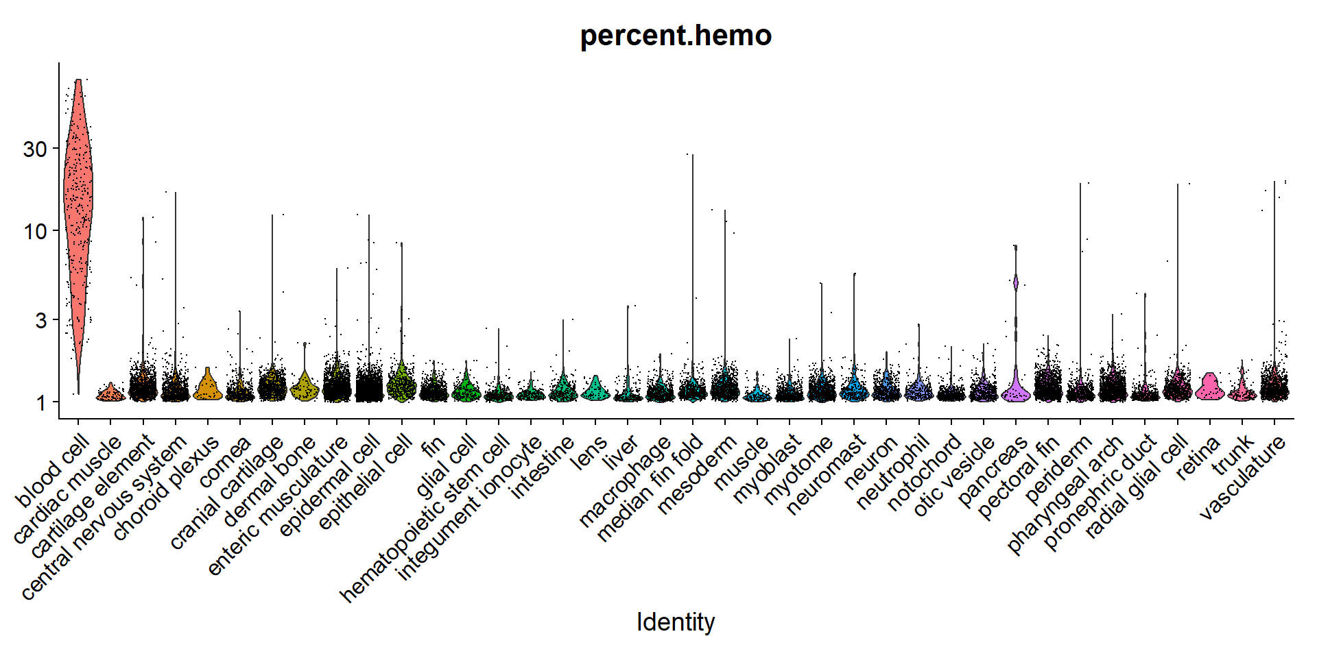

Parece que no hay tanta contaminación con células sanguíneas en el dataset

p2

Warning: Groups with fewer than two datapoints have been dropped.
ℹ Set `drop = FALSE` to consider such groups for position adjustment purposes.
Groups with fewer than two datapoints have been dropped.
ℹ Set `drop = FALSE` to consider such groups for position adjustment purposes.

Aca podemos ver claramente que el umbral de expresión usado para porcentaje mitocondrial es de 15%. Esto es por la gran variedad de tipos celulares: hay una cierta tendencia de las células más activas metabolicamente a expresar un mayor porcentaje de transcritos mitocondriales: higado, músculo y células que intercambian iones (pronephric e ionocitos).

VlnPlot(zf_atlas5dpf, "pct_counts_mt", group.by = "zebrafish_anatomy_ontology_class") + NoLegend()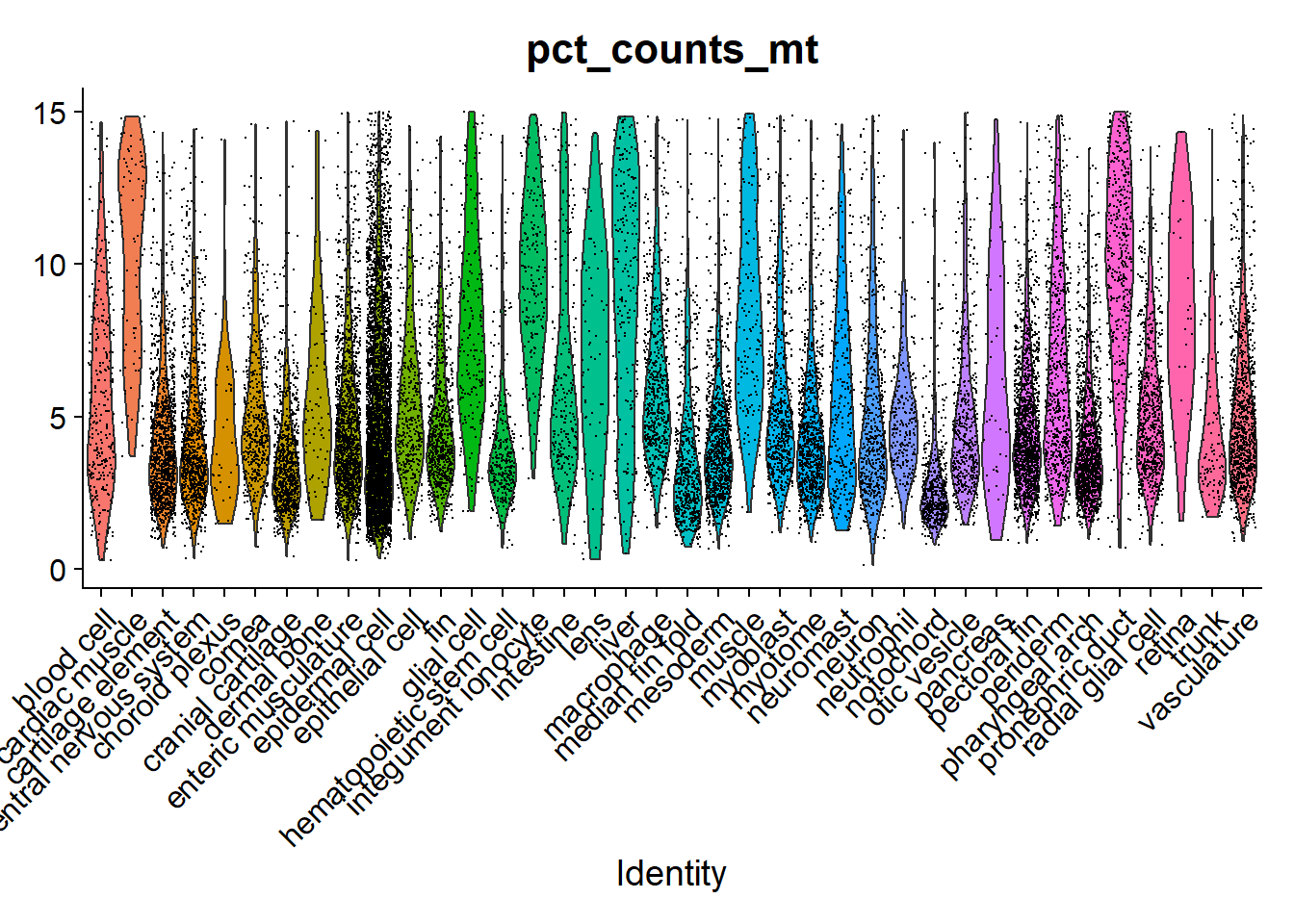

Quizas podriamos haber sido más laxos con nuestro filtro

VlnPlot(hc10x, "percent.mt", group.by = "predicted.id") + NoLegend()

Warning: Groups with fewer than two datapoints have been dropped.
ℹ Set `drop = FALSE` to consider such groups for position adjustment purposes.
Groups with fewer than two datapoints have been dropped.
ℹ Set `drop = FALSE` to consider such groups for position adjustment purposes.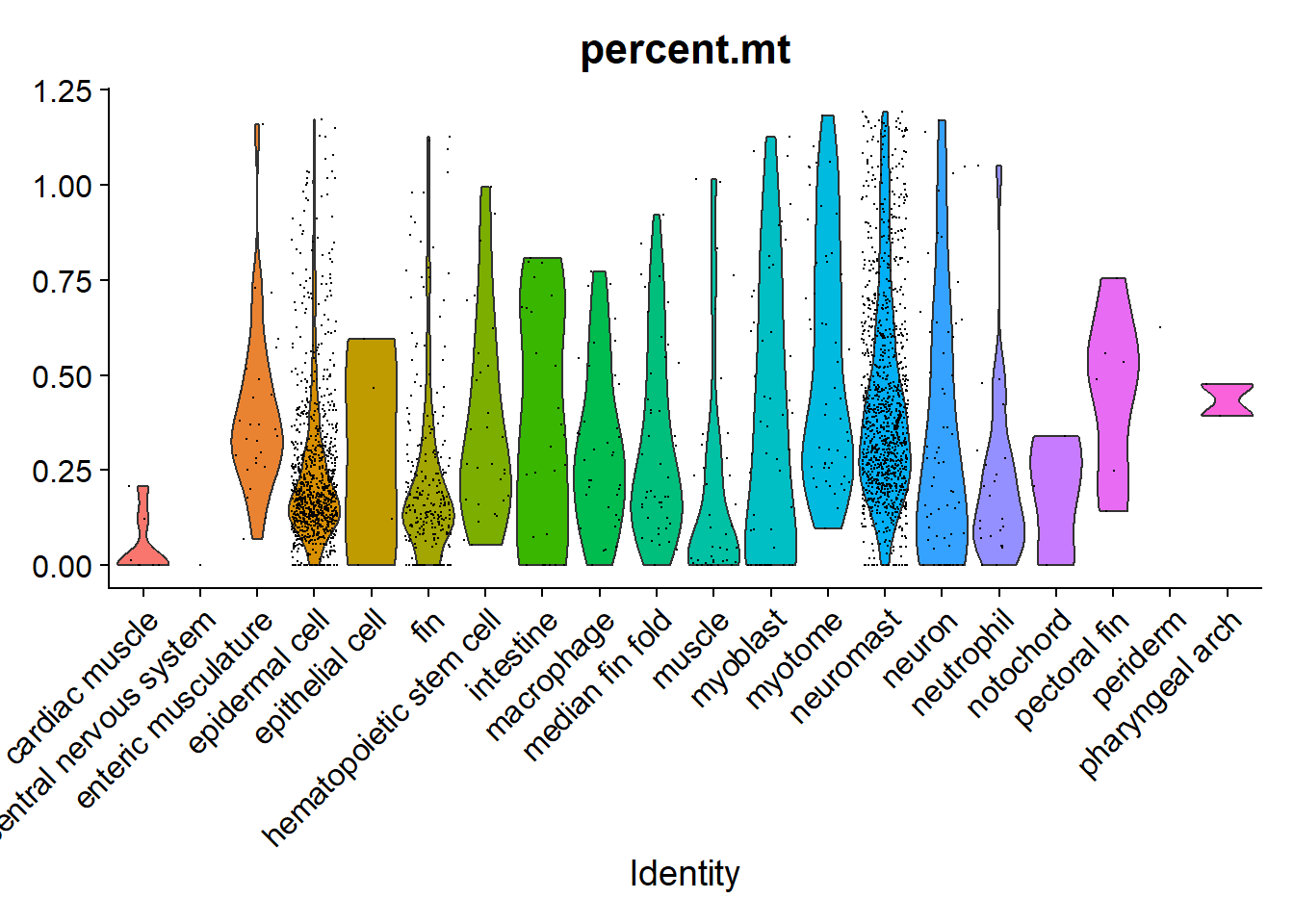

Integracion de dataset del neuromasto

Vamos a tomar de cada dataset solo las células anotadas como neuromasto, como este solo es un ejercicio por diversión, tomaremos tambien las células de neuromasto del atlas.

haircells10x <- subset(hc10x, subset = predicted.id == "neuromast")
##All scrb cells were neuromast cells
supportcells10x <- subset(sc10x, subset = predicted.id == "neuromast")
neuromast_atlas <- subset(zf_atlas5dpf, subset =  zebrafish_anatomy_ontology_class == "neuromast")

#Anadimos una columna de metadatos extra para distinguirlos despues de la integracion
supportcells10x$dataset <- rep("support",length(Cells(supportcells10x)))
hcSCRB$dataset <- rep("haircellSCRB",length(Cells(hcSCRB)))
neuromast_atlas$dataset <- rep("Atlas",length(Cells(neuromast_atlas)))
haircells10x$dataset <- rep("haircells10x", length(Cells(haircells10x)))
integrated <- c(neuromast_atlas, haircells10x, hcSCRB, supportcells10x)
anchors <- FindIntegrationAnchors(integrated)

Warning in CheckDuplicateCellNames(object.list = object.list): Some cell names
are duplicated across objects provided. Renaming to enforce unique cell names.

Computing 2000 integration features

Scaling features for provided objects

Warning: Different features in new layer data than already exists for
scale.data

Warning: Different features in new layer data than already exists for
scale.data
Warning: Different features in new layer data than already exists for
scale.data

Finding all pairwise anchors

Running CCA

Merging objects

Finding neighborhoods

Finding anchors

    Found 1318 anchors

Filtering anchors

    Retained 521 anchors

Running CCA

Merging objects

Finding neighborhoods

Finding anchors

    Found 849 anchors

Filtering anchors

Warning in FilterAnchors(object = object.pair, assay = assay, slot = slot, :
Number of anchor cells is less than k.filter. Retaining all anchors.

Running CCA

Merging objects

Finding neighborhoods

Finding anchors

    Found 918 anchors

Filtering anchors

Warning in FilterAnchors(object = object.pair, assay = assay, slot = slot, :
Number of anchor cells is less than k.filter. Retaining all anchors.

Running CCA

Merging objects

Finding neighborhoods

Finding anchors

    Found 849 anchors

Filtering anchors

Warning in FilterAnchors(object = object.pair, assay = assay, slot = slot, :
Number of anchor cells is less than k.filter. Retaining all anchors.

Running CCA

Merging objects

Finding neighborhoods

Finding anchors

    Found 946 anchors

Filtering anchors

Warning in FilterAnchors(object = object.pair, assay = assay, slot = slot, :
Number of anchor cells is less than k.filter. Retaining all anchors.

Running CCA

Merging objects

Finding neighborhoods

Finding anchors

    Found 760 anchors

Filtering anchors

Warning in FilterAnchors(object = object.pair, assay = assay, slot = slot, :
Number of anchor cells is less than k.filter. Retaining all anchors.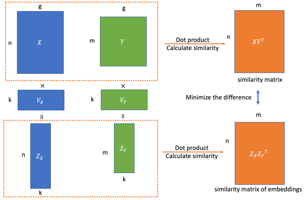

Integracion por Canonical Component Analysis

integrated <- IntegrateData(anchors, verbose = T)

Merging dataset 3 into 2

Extracting anchors for merged samples

Finding integration vectors

Finding integration vector weights

Integrating data

Warning: Layer counts isn't present in the assay object; returning NULL

Merging dataset 4 into 1

Extracting anchors for merged samples

Finding integration vectors

Finding integration vector weights

Integrating data

Warning: Layer counts isn't present in the assay object; returning NULL

Merging dataset 1 4 into 2 3

Extracting anchors for merged samples

Finding integration vectors

Finding integration vector weights

Integrating data

Warning: Layer counts isn't present in the assay object; returning NULL

DefaultAssay(integrated) <- "integrated"
integrated <- ScaleData(integrated)

Centering and scaling data matrix

#Variable features were calculated automatically
integrated <- RunPCA(integrated)

PC_ 1 
Positive:  pvalb8, cabp2b, gpx2, atp2b1a, otofb, si:ch211-255p10.3, gpx1b, s100t, calml4a, s100s 
       nptna, myo15ab, tmem240b, osbpl1a, tspan13b, si:ch211-145b13.5, tmc2b, atp1a3b, tekt3, si:dkeyp-72h1.1 
       anxa5a, rabl6b, wu:fj16a03, si:ch211-163l21.7, mt2, kif1aa, ptpn20, dnajc5b, zmp:0000001301, si:ch211-243g18.2 
Negative:  cldnb, si:dkey-205h13.2, si:ch211-195b11.3, phlda2, negaly6, junba, tmem176l.4, cd9b, si:dkey-4p15.5, krt1-c5 
       slc1a3a, cldnh, zgc:158343, zgc:162730, cbln20, elf3, zfp36l1b, soul5, tmsb4x, si:dkeyp-110c7.4 
       pdia3, krt8, apodb, cbln18, tmsb, btg2, si:dkey-33m11.8, rplp2l, egr2a, zgc:165423 
PC_ 2 
Positive:  wu:fj16a03, tmem176l.4, cbln18, s100s, cbln20, si:dkeyp-110c7.4, slc1a3a, soul5, negaly6, si:dkey-4p15.5 
       zgc:165423, si:dkey-33m11.8, si:dkey-205h13.2, glula, foxq1a, phlda2, si:ch211-255p10.3, apodb, soul2, zgc:162730 
       si:ch73-199e17.1, tmem176l.2, zfp36l1b, krt1-c5, zgc:158343, mb, tspan35, si:ch211-71m22.1, egr2a, cadm4 
Negative:  tuba1c, gstp1, rnf41l, tuba1a, ptmab, atoh1a, otofa, si:ch211-243g18.2, si:dkey-280e21.3, zgc:153665 
       si:ch211-114n24.6, shisa2a, capn8, jam2a, zgc:162989, pax2a, rplp0, hsp90ab1, camk2n1a, scg3 
       si:ch211-236g6.1, sh2d4bb, gipc3, espnlb, fxyd1, dld, nqo1, nap1l4b, anxa4, rbm24a 
PC_ 3 
Positive:  pvalb8, si:ch211-114n24.6, zgc:165423, osbpl1a, cbln18, gapdhs, si:dkey-4p15.5, tekt3, si:ch73-199e17.1, si:dkeyp-110c7.4 
       cbln20, gpx2, zgc:153911, s100t, nqo1, gpx1b, si:dkey-33m11.8, eno1a, nptna, tspan13b 
       slc1a3a, anxa5a, soul5, hbegfb, si:ch211-71m22.1, daw1, cd109, tmem176l.2, hsp70.1, si:dkey-222f2.1 
Negative:  si:ch211-222l21.1, krt91, si:ch211-236g6.1, pmp22a, cyt1, dld, rbp4, krtt1c19e, pfn1, and2 
       rnf41l, rplp2l, mycn, rpl23, rpl11, rps15a, cyt1l, col1a2, ppiaa, rpl29 
       zgc:136930, si:dkey-183i3.5, kdm6bb, rps9, jam2a, rps25, rsl1d1, rps21, dla, rps20 
PC_ 4 
Positive:  zgc:153665, otofa, atp1a1b, hsp70.1, gstp1, hsp70l, fxyd1, hsp70.3, nap1l4b, camk2n1a 
       si:ch211-195b15.8, zgc:153911, jdp2b, desma, fam131c, espnla, cd82a, dnajb1b, tbata, atp2b3b 
       krt5, degs2, zgc:193505, cxcl14, wu:fb18f06, fam228a, socs3a, ddit3, si:dkey-280e21.3, sh2d4bb 
Negative:  s100s, si:dkeyp-72h1.1, adcyap1b, si:ch211-255p10.3, wu:fj16a03, rabl6b, gramd2aa, atp6v1c2, cox5aa, si:ch211-222l21.1 
       hoxb7a, rnf41l, mt2, cabp2b, dld, spink4, atp1b1b, ptpdc1a, six2b, rbx1 
       atp1a3b, calm2a, ndufa4, ttll2, zgc:154006, tmem240b, aif1l, dla, eny2, snrpe 
PC_ 5 
Positive:  s100a10b, col1a1a, postnb, col1a2, col1a1b, pfn1, rbp4, si:dkey-248g15.3, krt91, cxl34b.11 
       eif4ebp3l, krt5, rplp0, hsp90ab1, cyt1l, cyt1, rpl22, lgals3b, atp1b3a, tmsb4x 
       eef1a1l1, zgc:136930, id1, ran, rpl10, rpl15, rpl39, pdlim1, tekt3, itgb4 
Negative:  dld, rnf41l, espnlb, zgc:171699, jam2a, atoh1a, shisa2a, kdm6bb, mtmr8, amer2 
       cldnh, scg3, dlb, sox1b, dla, tmsb, lfng, si:ch211-236g6.1, cxcr4b, marcksb 
       si:ch211-222l21.1, nuak1a, marcksl1b, tuba1c, otofa, pax2a, her4.2, tuba1a, lrrc73, eny2

integrated <- RunUMAP(integrated, reduction = "pca", , dims = 1:30)

10:56:04 UMAP embedding parameters a = 0.9922 b = 1.112

10:56:04 Read 1773 rows and found 30 numeric columns

10:56:04 Using Annoy for neighbor search, n_neighbors = 30

10:56:04 Building Annoy index with metric = cosine, n_trees = 50

0%   10   20   30   40   50   60   70   80   90   100%

[----|----|----|----|----|----|----|----|----|----|

**************************************************|
10:56:05 Writing NN index file to temp file C:\Users\mwaso\AppData\Local\Temp\RtmpmiAn33\file7a8c21ee6e6f
10:56:05 Searching Annoy index using 1 thread, search_k = 3000
10:56:06 Annoy recall = 100%
10:56:06 Commencing smooth kNN distance calibration using 1 thread with target n_neighbors = 30
10:56:07 Initializing from normalized Laplacian + noise (using RSpectra)
10:56:07 Commencing optimization for 500 epochs, with 75598 positive edges
10:56:17 Optimization finished

integrated <- FindNeighbors(integrated, dims = 1:30)

Computing nearest neighbor graph
Computing SNN

integrated <- FindClusters(integrated, resolution = 0.25)

Modularity Optimizer version 1.3.0 by Ludo Waltman and Nees Jan van Eck

Number of nodes: 1773
Number of edges: 84997

Running Louvain algorithm...
Maximum modularity in 10 random starts: 0.8227
Number of communities: 4
Elapsed time: 0 seconds

plot1 <- DimPlot(integrated, reduction = "umap", group.by = "dataset", pt.size = 2)
plot2 <- DimPlot(integrated, reduction = "umap", group.by = "seurat_clusters", label =T)
plot1 + plot2

Los clústers no parecen deberse a efectos de batch. Aunque el hecho de que hayamos enriquecido diferentes tipos celulares en cada dataset ya anticipa cuales células son haircells y cuales son support cells.

Expresión diferencial para encontrar marcadores

integrated.markers <- FindAllMarkers(integrated, only.pos = TRUE)  #función para encontrar todos los marcadores

Calculating cluster 0

Warning in mean.fxn(object[features, cells.1, drop = FALSE]): NaNs wurden
erzeugt

Warning in mean.fxn(object[features, cells.2, drop = FALSE]): NaNs wurden
erzeugt

For a (much!) faster implementation of the Wilcoxon Rank Sum Test,
(default method for FindMarkers) please install the presto package
--------------------------------------------
install.packages('devtools')
devtools::install_github('immunogenomics/presto')
--------------------------------------------
After installation of presto, Seurat will automatically use the more 
efficient implementation (no further action necessary).
This message will be shown once per session

Calculating cluster 1

Warning in mean.fxn(object[features, cells.1, drop = FALSE]): NaNs wurden
erzeugt
Warning in mean.fxn(object[features, cells.1, drop = FALSE]): NaNs wurden
erzeugt

Calculating cluster 2

Warning in mean.fxn(object[features, cells.1, drop = FALSE]): NaNs wurden
erzeugt
Warning in mean.fxn(object[features, cells.1, drop = FALSE]): NaNs wurden
erzeugt

Calculating cluster 3

Warning in mean.fxn(object[features, cells.1, drop = FALSE]): NaNs wurden
erzeugt
Warning in mean.fxn(object[features, cells.1, drop = FALSE]): NaNs wurden
erzeugt

#Cuantos marcadores hay por cluster
integrated.markers %>% group_by(cluster) %>% summarise(númerodemarcardores = n())

# A tibble: 4 × 2
  cluster númerodemarcardores
  <fct>                 <int>
1 0                       435
2 1                       691
3 2                       283
4 3                       635

byclustertop10markers <- integrated.markers %>% group_by(cluster) %>% 
  arrange(desc(avg_log2FC), .by_group = TRUE) %>% slice_head(n = 10) %>% pull(gene) %>% unique()
DotPlot(integrated, cols = c("lightgray", "red"), col.min = 0, features = byclustertop10markers, group.by = "seurat_clusters") + 
  theme(axis.text.x = element_text(angle = 45, hjust = 1))

Warning: Scaling data with a low number of groups may produce misleading
results

Anotacion de clusters

Seurat::DoHeatmap(integrated, features = c("negaly6", "stm",  "atoh1a", "myo6b", "tekt3", "pvalb8", "emx2"), group.by = "seurat_clusters", slot = "scale.data")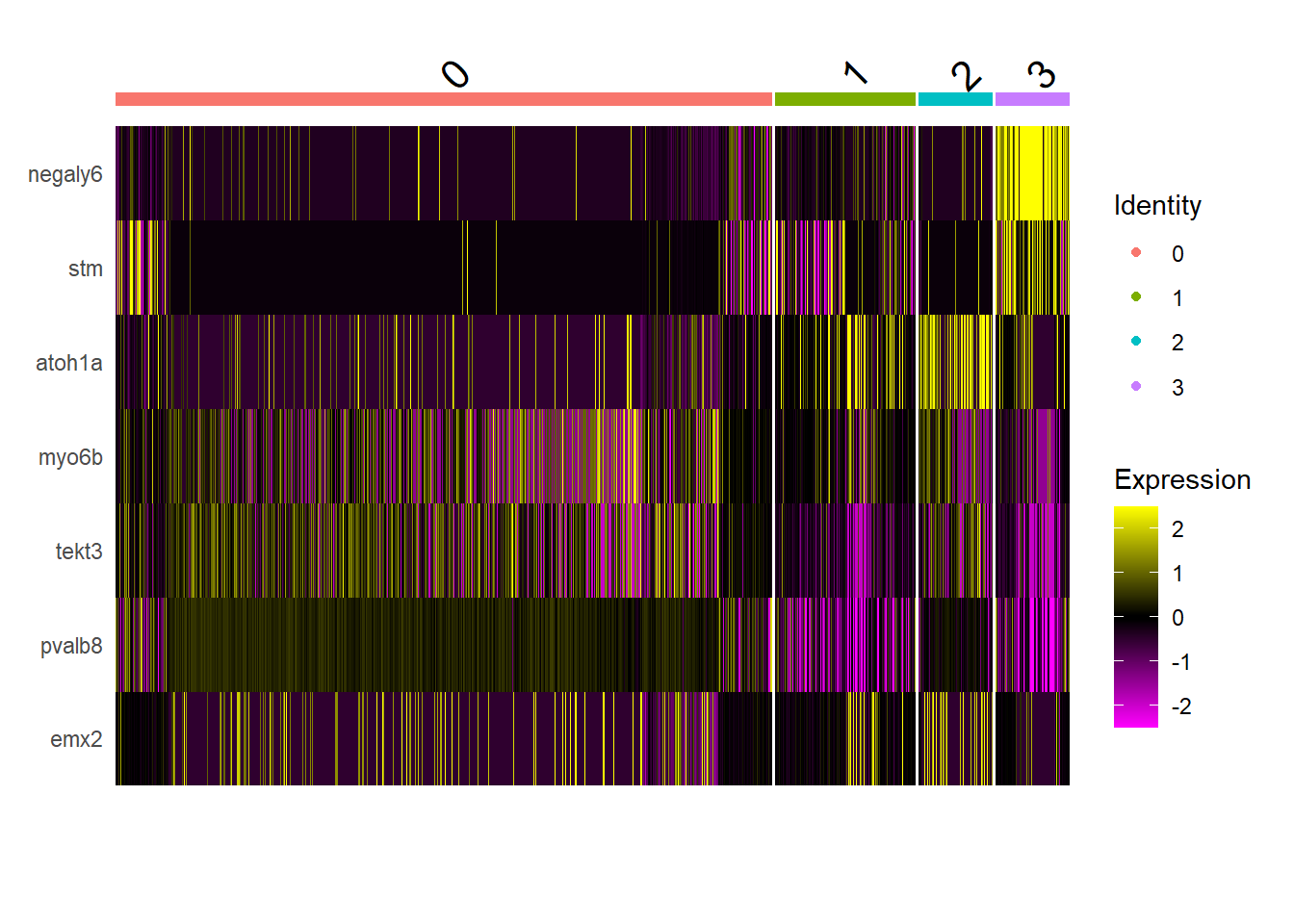

Como se compara con el heatmap publicado?

new.cluster.ids <- c("Hair_Cells", "Progenitors1", "Progenitors2", "Support_cells")
names(new.cluster.ids) <- levels(integrated)
integrated <- RenameIdents(integrated, new.cluster.ids)
DimPlot(integrated, reduction = "umap", label = TRUE, pt.size = 0.5) + NoLegend()

References

Bagnoli, Johannes W., Christoph Ziegenhain, Aleksandar Janjic, Lucas E. Wange, Beate Vieth, Swati Parekh, Johanna Geuder, Ines Hellmann, and Wolfgang Enard. 2018. “Sensitive and Powerful Single-Cell RNA Sequencing Using mcSCRB-Seq.” Nature Communications 9 (1): 2937. https://doi.org/10.1038/s41467-018-05347-6.

Kozak, Eva L., Subarna Palit, Jerónimo R. Miranda-Rodríguez, Aleksandar Janjic, Anika Böttcher, Heiko Lickert, Wolfgang Enard, Fabian J. Theis, and Hernán López-Schier. 2020. “Epithelial Planar Bipolarity Emerges from Notch-Mediated Asymmetric Inhibition of Emx2.” Current Biology 30 (6): 1142–1151.e6. https://doi.org/10.1016/j.cub.2020.01.027.

Xu, Chen, and Zhengchang Su. 2015. “Identification of Cell Types from Single-Cell Transcriptomes Using a Novel Clustering Method.” Bioinformatics 31 (12): 1974–80. https://doi.org/10.1093/bioinformatics/btv088.

Footnotes

Los archivos fastq fueron alineados a una referencia splice+i. Es decir, una referencia del transcriptoma más intrones. Utilizando el pipeline de simpleaf con el transcriptoma del pez cebra al que se le anadio la secuencia de EGFP utilizada en transgenicos. Este pipeline tambien se encarga de resolver los UMIS y los barcodes. https://simpleaf.readthedocs.io/en/latest/↩︎